19.1: Belief, probability and odds

For instance, we want to formulate the following
"probability":
$(A):$
the " probability"
that
Japan will win
the victory in
the next
FIFA World Cup
This is possible (cf. ref. [8] in $\S$0.0), if
" parimutuel betting
( or,
odds in bookmaker
)"
is
formulated by
Axiom$^{(m)}$ 1
(
mixed measurement
).
The purpose of this chapter
is
to show it,
and further,
to
propose the principle of equal weight,
that
is,
whose justice
is not solved yet.
That is, it is one of the most important unsolved problems in statistics.
$(B):$
the principle that, in the absence of any reason to expect one event rather than another, all the possible events should be assigned the same probability}.
In Chapter 9, we studied the mixed measurement: that is,
\[ \underset{\mbox{ (=quantum language)}}{\fbox{mixed measurement theory (A)}} := \underbrace{ \color{red}{ \underset{\mbox{ (\(\S\)9.1)}}{ \overset{ [\mbox{ (mixed) Axiom 1}] }{\fbox{mixed measurement}} } } + \underset{\mbox{ ( \(\S \)10.3)}}{ \overset{ [{\mbox{ Axiom 2}}] }{\fbox{Causality}} } }_{\mbox{ a kind of incantation (a priori judgment)}} + \underbrace{ \underset{\mbox{ (\(\S\)3.1) }} { \overset{ {}}{\fbox{Linguistic interpretation}} } }_{\mbox{ the manual on how to use spells}} \tag{9.2} \]
The purpose of this chapter is to characterize "belief" as a kind of mixed measurement.
19.1.1: A simple example; how to describe "belief" in quantum language
We begin with a simplest example (cf. Problem 9.5) as follows.
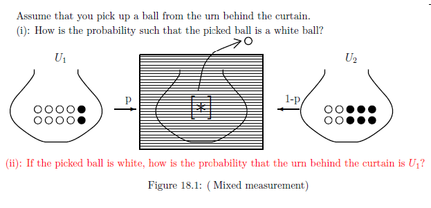
| $(C):$ | You do not know which the urn behind the curtain is, $U_1$ or $U_2$, but the "probability": $p$ and $1-p$. |
Answer 19.2 (=Answer 9.13)
Put $\Omega=\{ \omega_1, \omega_2 \}$ with the discrete metric and the counting measure $\nu_c$, thus, note that $C_0(\Omega)$ $=C(\Omega )$ $= L^\infty (\Omega, \nu )$. Thus, in this chapter, we devote ourselves to the $C^*$-algebraic formulation: Define the observables ${\mathsf O} = ( \{ {{{W}},} {{B}} \},$ $ 2^{\{ {{W}}, {{B}} \} } ,$ $ F)$ and ${\mathsf O}_U = ( \{ {{{U_1}},} {{U_2}} \},$ $ 2^{\{ {{U_1}}, {{U_2}} \} } ,$ $ G_U)$ in $C(\Omega)$ by \begin{align} & F(\{ {{W}} \})(\omega_1)= 0.8, F(\{ {{B}} \})(\omega_1)= 0.2, F(\{ {{W}} \})(\omega_2)= 0.4, F(\{ {{B}} \})(\omega_2)= 0.6 \\ & G_U(\{ {{U_1}} \})(\omega_1)= 1, G_U(\{ {{U_2}} \})(\omega_1)= 0, G_U(\{ {{U_1}} \})(\omega_2)= 0, G_U(\{ {{U_2}} \})(\omega_2)= 1 \end{align}
Here "$W$" and "$B$" means "white" and "black" respectively. Under the identification: $U_1 \approx \omega_1$ and $U_2 \approx \omega_2$, the above situation is represented by the mixed state $\rho^{(p)}_{\mbox{ prior}} ( \in {\mathcal M}_{+1} (\Omega))$ such that \begin{align} \rho^{(p)}_{\mbox{ prior}} = p \delta_{\omega_1} + (1-p) \delta_{\omega_2} \end{align} where $\delta_{\omega}$ is the point measure at $\omega$. Thus, we have the mixed measurement: \begin{align} {\mathsf M}_{C (\Omega)}({\mathsf O} \times {\mathsf O}_{U} := ( \{ {{{W}},} {{B}} \} \times \{U_1, U_2\} ,2^{ \{ {{{W}},} {{B}} \} \times \{U_1, U_2\} } , F \times G_U), S_{[*]}( \rho^{(p)}_{\mbox{ prior}} )) \tag{19.2} \end{align}
Axiom${}^{(m)}$ 1 gives the answer to the (i) in Problem 19.1 as follows.
| $(D):$ | the probability that a measured value $(x,y) $ obtained by the mixed measurement ${\mathsf M}_{C (\Omega)}({\mathsf O} \times {\mathsf O}_{U}, S_{[*]}( \rho^{(p)}_{\mbox{ prior}} ))$ belongs to $\{W \} \times \{U_1, U_2 \}$ is given by $$ {}_{{\mathcal M}(\Omega)}(\rho^{(p)}_{\mbox{ prior}}, F(\{W\}) )_{C_{}(\Omega )} = 0.8 p + 0.4 (1-p). $$ |
Since a white ball is obtained, Answer 9.13Answer} (=Bayes' theorem ) says that a new {mixed state} $\rho^{(p)}_{\mbox{ post}} (\in {\mathcal M}_{+1}(\Omega ))$ is given by
\begin{align} \rho^{(p)}_{\mbox{ post}} & = \frac{ F(\{ {{W}}\} ) \rho^{(p)}_{\mbox{ prior}} }{\int_\Omega [F( \{ {{W}}\} )](\omega) \rho^{(p)}_{\mbox{ prior}}(d \omega )} = \frac{\displaystyle 0.8 p }{\displaystyle 0.8p+0.4(1-p) } \delta_{\omega_1} + \frac{\displaystyle 0.4(1- p) }{\displaystyle 0.8p+0.4(1-p) } \delta_{\omega_2} \tag{19.3} \end{align} Hence, the answer of the (ii) is given by $$ {}_{{\mathcal M}(\Omega)}(\rho^{(p)}_{\mbox{ post}}, G_U(\{ U_1 \}) )_{C_{}(\Omega )} = \frac{\displaystyle 0.8 p }{\displaystyle 0.8p+0.4(1-p) } $$
By an analogy of the above Problem 19.1Problem}
( for simplicity, we put:
$
p=1/4, \;\; 1-p = 3/4
$
),
we consider as follows.
Assume that
there are 100 people. And moreover assume the following sitiation
(E) such that,
for some reasons,
Now, we have the following problem:
Problem 19.3 Consider Situation (E) and Situation (C) ( $ p=1/4, \;\; 1-p = 3/4 $ ). Then,
| $(F_1):$ | Can Situation (E) be understood like Situation (C) ? |
| $(F_2):$ | Can Situation (E) be formulated in mixed measurement (i.e., Axiom${}^{(m)}$ 1)? $\;\;\;$ That is, can Situation (E) be described in quantum language? |
19.1.2: The affirmative answer to Problem 19.3.
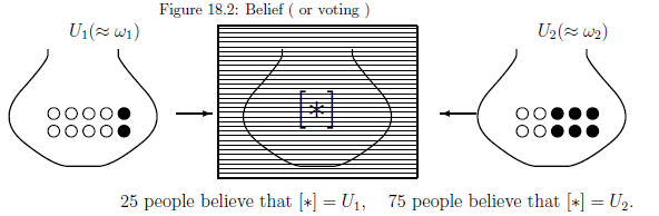
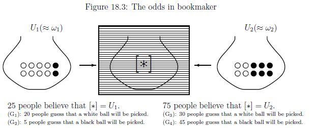
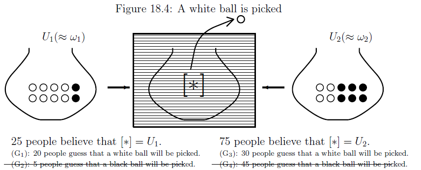
Since 100 people know the situation of the urn (i.e., Figure 19.2, the assumption (E) ) implies (G)(=Figure 19.3), that is,
| $(G):$ | $ \left\{\begin{array}{ll} \mbox{25 people (in 100 people) believe that $[\ast]= U_1$} \\ \quad \Longrightarrow \left\{\begin{array}{ll} \mbox{(G$_1$): 20 people guess (or bet) that a white ball will be picked} \\ \mbox{(G$_2$): 5 people guess (or bet) that a black ball will be picked} \end{array}\right. \\ \mbox{75 people (in 100 people) believe that $[\ast]= U_2$} \\ \quad \Longrightarrow \left\{\begin{array}{ll} \mbox{(G$_3$): 30 people guess (or bet) that a white ball will be picked} \\ \mbox{(G$_4$): 45 people guess (or bet) that a black ball will be picked} \end{array}\right. \end{array}\right. $ |
Assume that a white ball is picked in the above figure. Then, the above (G$_2$) and (G$_4$) are vanished as follows.
After all, we get the following figure:
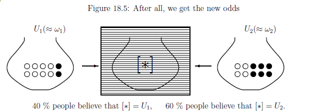
Thus we see that \begin{align} \overset{{\mbox{ (prior state)}}}{\underset{\frac{1}{4} \delta_{\omega_1} + \frac{3}{4} \delta_{\omega_2}}{\fbox{Fig. 19.3}}} \xrightarrow[{\mbox{$\qquad \qquad$}}]{} \overset{{\mbox{ (a white ball is picked)}}}{\fbox{Fig. 19.4}} \xrightarrow[{\mbox{$\qquad \qquad$}}]{} \overset{{\mbox{ (post state)}}}{\underset{\frac{2}{5} \delta_{\omega_1} + \frac{3}{5} \delta_{\omega_2}}{\fbox{Fig.19.5}}} \tag{19.4} \end{align}
Considering the mixed measurement (i.e., the (19.2) in the case that $p=1/4$, $1-p=3/4$ ):
\begin{align} {\mathsf M}_{C_{} (\Omega)}({\mathsf O} \times{\mathsf O}_U = ( \{ {{{W}},} {{B}} \} \times \{U_1, U_2\},2^{ \{ {{{W}},} {{B}} \} \times \{U_1, U_2\} } , F\times G_U) , S_{[*]}( \rho^{(1/4)}_{\mbox{ prior}} )) \tag{19.5} \end{align} we see that the above (19.4) is the same as the Bayesian result (19.3).Note that the measurement (8.5) is interpreted as
| $(H):$ | choose one person from the 100 people at random, and ask him/her "Do you guess that a white ball (or, a black ball) will be picked from the urn behind the curtain, and its urn is $U_1$ or $U_2$?" |
In what follows, let us explain it. Consider the product observable $ \widehat{\mathsf O} \times \widehat{\mathsf O}_{U} $ of $\widehat{\mathsf O}= ( \{W,B \}, 2^{\{W,B \} },$ $ \widehat{F})$ and $\widehat{\mathsf O}_{U}= ( \{U_1, U_2 \}, 2^{\{U_1, U_2 \} }, \widehat{G}_U)$ in $C(\Theta)$ (where $\Theta=\{ \theta_1, \theta_2, ..., \theta_{100} \}$) such that
\begin{align} & [\widehat{F} (\{W\})](\theta_k)=4/5,\;\; [\widehat{F}(\{B\})](\theta_k)=1/5, \;\; (k=1,2,...,25) \nonumber \\ & [\widehat{F}(\{W\})](\theta_k)=2/5,\;\; [\widehat{F}(\{B\})](\theta_k)=3/5, \;\; (k=26,27,...,100) \tag{19.6} \\ & [\widehat{G}_{U}(\{ U_1 \})](\theta_k)=1,\;\; [\widehat{G}_{U}(\{ U_2 \})](\theta_k)=0, \;\; (k=1,2,...,25) \nonumber \\ & [\widehat{G}_{U}(\{ U_1 \})](\theta_k)=0,\;\; [\widehat{G}_{U}(\{ U_2 \})](\theta_k)=1, \;\; (k=26,27,...,100) \tag{19.7} \end{align}And put $\nu_0= (1/100) \sum_{k=1}^{100} \delta_{\theta_k} (\in {\mathcal M}_{+1}(\Theta))$. Then, the above measurement (H) is formulated by
\begin{align} {\mathsf M}_{C_{} (\Theta)}(\widehat{\mathsf O} \times \widehat{\mathsf O}_U = ( \{ {{{W}},} {{B}} \} \times \{U_1, U_2\},2^{ \{ {{{W}},} {{B}} \} \times \{U_1, U_2\} } , \widehat{F} \times \widehat{G}_U) , S_{[*]}( \nu_0 )) \tag{19.8} \end{align}which is identified with the measurement (19.5) under the deterministic causal operator $\Phi:C(\Omega) \to C(\Theta)$ such that $\Phi^* (\delta_{\theta_k} ) =\delta_{\omega_1}$ $(k=1,2,...,25)$, $ =\delta_{\omega_2}\; (k=26,27,...,100)$. That is, we see, symbolically,
$$ \fbox{(19.8): the Heisenberg picture} \xleftarrow[\mbox{ identification}]{\Phi} \fbox{(19.5): the Schrödinger picture} $$ Thus, we can answer Problem 19.3 such that| $(I_1):$ | Situation (E) can be understood like Situation (C). |
| $(I_2):$ | Situation (E) can be formulated in mixed measurement (i.e., Axiom${}^{(m)}$ 1). $\;\;\;$ In the same sense, Situation (E) can be described in quantum language. |
