11.1: The Heisenberg picture and the Schrödinger picture
11.1.1: State does not move--- the Heisenberg picture ---
We consider that
That is because
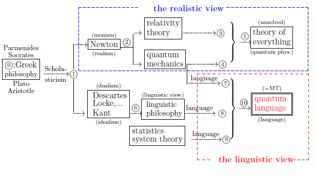 |
| $\qquad \quad $Fig. 1.1: The history of world-descriptions |
| $(a):$ | In order to see the state movement, we have to take measurement at least more than twice. However, the "plural measurement" is prohibited. Thus, we conclude "state does not move" |
We want to believe that this is associated with Parmenides' words:
Theorem 11.1 [Causal operator and observable] Consider the basic structure: \begin{align} [ {\mathcal A}_k \subseteq \overline{\mathcal A}_k \subseteq {B(H_k)}] \qquad (k=1,2) \end{align} Let $\Phi_{1,2}:\overline{\mathcal A}_2 \to \overline{\mathcal A}_1$ be a causal operator, and let $ {\mathsf O}_2$ $=$ $(X , {\cal F} , F_2)$ be an observable in ${\overline{\mathcal A}_2}$. Then, $\Phi_{1,2} {\mathsf O}_2$ $=$ $(X , {\cal F} , \Phi_{1,2} F_2)$ is an observable in ${\overline{\mathcal A}_2}$.
Proof. Let $\Xi$ $(\in {\cal F} )$. And consider the countable decomposition $\{\Xi_1, \Xi_2, \ldots, \Xi_n, \ldots\}$ of $\Xi$ $\Big($ i.e., $\Xi = \bigcup\limits_{n=1}^\infty \Xi_n $, $\Xi_n \in {\cal F}, (n = 1, 2, \ldots)$, $\Xi_m \cap \Xi_n =\emptyset \;\; (m \not= n )$ $\Big)$. Then we see, for any $\rho_1 (\in ({{\mathcal A}_1})_*)$, \begin{align} & {}_{\stackrel{{}}{(\overline{\mathcal A}_1)_* }}\Big(\rho_1, \Phi_{1,2} F_2( \bigcup\limits_{n=1}^\infty \Xi_n ) \Big){}_{\stackrel{{}}{\overline{\mathcal A}_1 }} = {}_{\stackrel{{}}{(\overline{\mathcal A}_1)_* }}\Big( ({\Phi}_{1,2})_* \rho_1, F_2 ( \bigcup\limits_{n=1}^\infty \Xi_n ) \Big){}_{\stackrel{{}}{\overline{\mathcal A}_2 }} \\ = & \sum\limits_{n=1}^\infty {}_{\stackrel{{}}{(\overline{\mathcal A}_1)_* }}\Big( ({\Phi}_{1,2})_* \rho_1, F_2 ( \Xi_n ) \Big){}_{\stackrel{{}}{\overline{\mathcal A}_2 }} = \sum\limits_{n=1}^\infty {}_{\stackrel{{}}{(\overline{\mathcal A}_1)_* }}\Big( \rho_1, {\Phi}_{1,2} F_2 ( \Xi_n ) \Big){}_{\stackrel{{}}{\overline{\mathcal A}_2 }} \end{align} Thus,$\Phi_{1,2} {\mathsf O}_2$ $=$ $(X , {\cal F} , \Phi_{1,2} F_2)$ is an observable in $ \overline{\mathcal A}_1 $.
Let us begin from the simplest case. Consider a tree $T=\{0,1\}$. For each $t \in T$, consider the basic structure:
\begin{align} [ {\mathcal A}_t \subseteq \overline{\mathcal A}_t \subseteq {B(H_t)}] \qquad (t=0,1) \end{align}And consider the causal operator $\Phi_{0,1}: \overline{\mathcal A}_1 \to \overline{\mathcal A}_0$. That is,
\begin{align} \overline{\mathcal A}_0 \xleftarrow[]{\Phi_{0,1}} \overline{\mathcal A}_1 \tag{11.2} \end{align}Therefore, we have thepre-dual operator $(\Phi_{0,1})_*$ and the dual operator $\Phi_{0,1}^* $:
\begin{align} (\overline{\mathcal A}_0)_* \xrightarrow[(\Phi_{0,1})_*]{} (\overline{\mathcal A}_1)_* \qquad \qquad {\mathcal A}_0^* \xrightarrow[\Phi_{0,1}^*]{} {\mathcal A}_1^* \tag{11.3} \end{align}If $\Phi_{0,1}: \overline{\mathcal A}_1 \to \overline{\mathcal A}_0$ is deterministic, we see that
\begin{align} {\mathcal A}_0^* \supset {\frak S}^p{({\mathcal A}_0^*)} \ni \rho \xrightarrow[\Phi_{0,1}^*]{} \Phi_{0,1}^* \rho \in {\frak S}^p{({\mathcal A}_1^*)} \subset {\mathcal A}_1^* \tag{11.4} \end{align}Under the above preparation,we will explain the Heisenberg picture and the Schrödinger picture in what follows.
Assume that
| $(A_1):$ | Consider a deterministic causal operator $\Phi_{0,1}: \overline{\mathcal A}_1 \to \overline{\mathcal A}_0$. |
| $(A_2):$ | a state $\rho_{{}0}$ $ \in {\frak S}^p({\mathcal A}_{{}0}^*):\;\; \mbox{pure state} $ |
| $(A_3):$ | Let ${\mathsf O}_1=(X_1, {\mathcal F}_1, F_1)$ be an observable in $\overline{\mathcal A}_1$. |
| $(a1):$ | To identify an observable ${\mathsf O}_1$ in $\overline{\mathcal A}_1$ with an $\Phi_{0,1}{\mathsf O}_1$ in $\overline{\mathcal A}_0$ }. That is, \begin{align} \underset{\mbox{ ( in $\overline{\mathcal A}_0$)}}{\Phi_{0,1}\overline{\mathsf O}_1} \qquad \xleftarrow[\scriptsize{\mbox{ identification}}]{\Phi_{0,1}} \qquad \underset{\mbox{ ( in $\overline{\mathcal A}_1$)}}{{\mathsf O}_1} \end{align} |
| $(a2):$ | a measurement of an observable ${\mathsf O}_1$ (at time $t=1$) for a pure state $\rho_{{}0}$ (at time $t=0$) $ \in {\frak S}^p({\mathcal A}_{{}0}^*)$ is represented by \begin{align} {\mathsf M_{\overline{\mathcal A}_0}(\Phi_{0,1}{\mathsf O}_1}, S_{[\rho_0]}) \end{align} |
| $(a3):$ | the probability that a measured value belongs to $\Xi( \in {\mathcal F})$ is given by \begin{align} {}_{{\mathcal A}_0^* } \Big(\rho_0, \Phi_{0,1}(F_1( \Xi )) \Big) {}_{\overline{\mathcal A}_0} \tag{11.5} \end{align} |
| $(b1):$ | To identify a pure state $\Phi_{0,1}^* \rho_0 (\in {\frak S}^p({\mathcal A}_1^*))$ with $\rho_0 (\in {\frak S}^p({\mathcal A}_0^*))$, That is, \begin{align} {\mathcal A}_0^* \supset {\frak S}^p{({\mathcal A}_0^*)} \ni \rho_0 \xrightarrow[\scriptsize{\mbox{ identification}}]{\Phi_{0,1}^*} \Phi_{0,1}^* \rho_0 \in {\frak S}^p{({\mathcal A}_1^*)} \subset {\mathcal A}_1^* \nonumber \end{align} |
| $(b2):$ | a measurement of an observable ${\mathsf O}_1$ (at time $t=1$) for a pure state $\rho_{{}0}$ (at time $t=0$) $ \in {\frak S}^p({\mathcal A}_{{}1}^*)$ is represented by \begin{align} {\mathsf M_{\overline{\mathcal A}_1}({\mathsf O}_1}, S_{[\Phi_{0,1}^* \rho_0]}) \end{align} |
| $(a3):$ | the probability that a measured value belongs to $\Xi( \in {\mathcal F})$ is given by \begin{align} {}_{{\mathcal A}_1^* } \Big(\Phi_{0,1}^*\rho_0, F_1( \Xi ) \Big) {}_{\overline{\mathcal A}_1} \tag{11.6} \end{align} which is equal to \begin{align} {}_{{\mathcal A}_0^* } \Big(\rho_0, \Phi_{0,1}(F_1( \Xi )) \Big) {}_{\overline{\mathcal A}_0} \tag{11.7} \end{align} |
In the above sense (i.e., (11.6) and (11.7) ), we conclude that, under the condition (A$_1$), \begin{align} \mbox{ the Heisenberg picture and the Schrödinger picture are equivalent} \end{align} That is, \begin{align} \underset{\mbox{ (Heisenberg picture)}}{ \fbox{${\mathsf M_{\overline{\mathcal A}_0}(\Phi_{0,1}{\mathsf O}_1}, S_{[\rho_0]})$} } \quad \underset{\scriptsize{\mbox{ (identification)}}}{\longleftrightarrow} \quad \underset{\mbox{ (Schrödinger picture)}}{ \fbox{ ${\mathsf M_{\overline{\mathcal A}_1}({\mathsf O}_1}, S_{[\Phi_{0,1}^* \rho_0]}) $ } } \tag{11.8} \end{align}
| $(A_1):$ | Consider a deterministic causal operator $\Phi_{0,1}: \overline{\mathcal A}_1 \to \overline{\mathcal A}_0$. |
Without the deterministic conditions (A$_1$), the Schrödinger picture can not be formulated completely. That is because $ \Phi_{0,1}^* \rho_0 $ is not necessarily a pure state. On the other hand, the Heisenberg picture is always formulated. Hence we consider that we consider that
| $\bullet$ | $\left\{\begin{array}{ll} \mbox{ the Heisenberg picture is $\color{red}{formal}$} \\ \\ \mbox{ the Schrödinger picture is $\color{blue}{makeshift}$ } \end{array}\right. $ |
