10.4: Kinetic equation (in classical mechanics and quantum mechanics)
In this section, we consider the simplest
kinetic equation in
classical system
and
quantum system.
Consider the state space
$\Omega$ such that
$\Omega ={\mathbb R}^2$,
that is,
Hamiltonian ${\mathcal H}(q,p)$ is defined by the total energy,
for example,
as the typical case
($m$: particle mass), we consider that
Concerning
Hamiltonian
${\cal H}(q,p)$,
Hamilton's canonical equation
is defined by
And thus, in the case of (10.15}), we get
which is the same as Newtonian equation.
That is,
Now,
let us describe the above (10.17) in terms of quantum language.
For each
$ t \in T={\mathbb R}$,
define the
state space $\Omega_t$
by
and assume Lebesgue measure $\nu$.
Then, we have the classical basic structure:
The solution of the canonical
equation
(10.17)
is defined by
Since (10.19)
determines the deterministic causal map,
we have the deterministic sequential causal operator
$\{ \Phi_{t_1, t_2} : L^\infty (\Omega_{t_2} ) \to L^\infty (\Omega_{t_1} )$
$ \}_{(t_1, t_2 )\in T^2_{\le}}$
such that
The quantization
is the following procedure:
And therefore, we get the
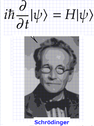
Schrödinger equation
:
Putting
$u(t, \cdot )=u_t \in L^2({\mathbb R} )$
$(\forall t \in T={\mathcal R})$
we denote the Schrödinger equation (10.23)
by
Newtonian equation(=Hamilton's canonical equation)
10.4.3: Schrödinger equation (quantizing Hamiltonian)
Solving this formally, we see
\begin{align} u_t = e^{\frac{\mathcal H}{\hbar \sqrt{-1}}t}u_0 \quad \mbox{ (Thus, the state representation is $|u_t \rangle \langle u_t| = |e^{\frac{\mathcal H}{\hbar \sqrt{-1}}t}u_0 \rangle \langle e^{\frac{\mathcal H}{\hbar \sqrt{-1}}t}u_0|$ } ) \tag{10.24} \end{align}where,$u_0 \in L^2({\mathbb R} )$ is an initial condition.
Now,put Hilbert space $H_t=L^2({\mathbb R})$ $(\forall t \in T={\mathbb R})$, and consider the quantum basic structure:
\begin{align} [ {\mathcal C}(L^2({\mathbb R})) \subseteq B(L^2({\mathbb R})) \subseteq B(L^2({\mathbb R})) ] \end{align}The dual sequential causal operator $\{ \Phi_{t_1, t_2}^* : {\mathcal Tr}(H_{t_1}) \to {\mathcal Tr}(H_{t_2}) \}_{(t_1, t_2 )\in T^2_{\le}}$ is defined by
\begin{align} \Phi_{t_1, t_2}^* (\rho)=e^{\frac{\mathcal H}{\hbar \sqrt{-1}}(t_2-t_1)} \rho e^{\frac{-{\mathcal H}}{\hbar \sqrt{-1}}(t_2-t_1)} \quad (\forall \rho \in {\mathcal Tr}(H_{t_1}) = (B(H_{t_1}))_* = {\mathcal C}(H_{t_1})^*) \tag{10.25} \end{align}And therefore, { the sequential causal operator $\{ \Phi_{t_1, t_2} : B(H_{t_2}) \to B(H_{t_1}) \}_{(t_1, t_2 )\in T^2_{\le}}$ is defined by
\begin{align} \Phi_{t_1, t_2} (A)=e^{\frac{-{\mathcal H}}{\hbar \sqrt{-1}}(t_2-t_1)} A e^{\frac{{\mathcal H}}{\hbar \sqrt{-1}}(t_2-t_1)} \quad (\forall A \in B(H_{t_2})) \tag{10.26} \end{align}} Also, since
\begin{align} \Phi_{t_1, t_2}^*( {\frak S}^p({\mathcal C}(H_{t_1})^* ) ) \subseteq {\frak S}^p({\mathcal C}(H_{t_2})^* ), \end{align}the sequential causal operator $\{ \Phi_{t_1, t_2} : B(H_{t_2}) \to B(H_{t_1}) \}_{(t_1, t_2 )\in T^2_{\le}}$ is deterministic. Since we deal with the time-invariant system, putting $t=t_2-t_1$, we see that (10.26) is equal to
\begin{align} A_t=\Phi_t(A_0)= e^{\frac{-{\mathcal H}}{\hbar \sqrt{-1}}t} A_0 e^{\frac{{\mathcal H}}{\hbar \sqrt{-1}}t} \tag{10.27} \end{align}And thus, we get the differential equation:
\begin{align} \frac{dA_t}{dt} &= \frac{-{\mathcal H}}{\hbar \sqrt{-1}} e^{\frac{-{\mathcal H}}{\hbar \sqrt{-1}}t} A_0 e^{\frac{{\mathcal H}}{\hbar \sqrt{-1}}t} + \frac{-{\mathcal H}}{\hbar \sqrt{-1}} e^{\frac{-{\mathcal H}}{\hbar \sqrt{-1}}t} A_0 e^{\frac{{\mathcal H}}{\hbar \sqrt{-1}}t}\frac{{\mathcal H}}{\hbar \sqrt{-1}} \nonumber \\ &= \frac{-{\mathcal H}}{\hbar \sqrt{-1}}A_t + A_t\frac{{\mathcal H}}{\hbar \sqrt{-1}} = \frac{1}{\hbar \sqrt{-1}} \Big( A_t {\mathcal H} - {\mathcal H}A_t \Big) \tag{10.28} \end{align}which is just Heisenberg's kinetic equation. In quantum lanuage, we say that
| $(\sharp)$ | Heisenberg's kinetic equation is formal, and Schrödinger equation is makeshift. |
