In classical mechanics, the term "observable" usually means the continuous real valued function on a state space (that is, physical quantity).
An observable in measurement theory (= quantum language ) is characterized as the natural generalization of the physical quantity. This will be explained in the following examples.
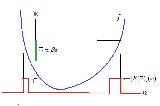
Example 2.26 [System quantity] Let $[C_0(\Omega ) \subseteq L^\infty (\Omega, \nu ) \subseteq B(L^2 (\Omega, \nu ))]$ be the classical basic structure. A continuous real valued function ${\widetilde f}{}: \Omega \to {\mathbb R}$ ( or generally, a measurable ${\mathbb R}^n$-valued function ${\widetilde f}{}: \Omega \to {\mathbb R}^n$) is called a system quantity (or in short, quantity) on $\Omega$. Define the projective observable ${\mathsf O}=({}{\mathbb R}, {\cal B}_{\mathbb R} , F{})$ in ${L^\infty ( \Omega, \nu )}$ such that
\begin{align*} [{}F({}\Xi{})] (\omega) = \left\{ \begin{array}{l} 1 \quad \mbox{when } \omega \in {\widetilde f}^{-1}({}\Xi{}) \ \\ \\ 0 \quad \mbox{when } \omega \notin {\widetilde f}^{-1}({}\Xi{}) \end{array} \right. \qquad ( \forall \Xi \in {\cal B}_{\mathbb R} ) \end{align*} Here, note that \begin{align} {\widetilde f} (\omega) = \lim_{N \to \infty } \sum\limits_{n=-N^2}^{N^2} \frac{n}{N} \left[F \bigm( [\frac{n}{N},\frac{n+1}{N} ) \bigm) \right](\omega) = \int_{\mathbb R} \lambda [F({}d \lambda{}) ](\omega) \qquad \tag{2.59} \end{align} Thus, we have the following identification: \begin{align} \underset{{\mbox{ (system quantity on $\Omega$)}}}{{\widetilde f}} {{\longleftrightarrow}} \underset{{\mbox{ (projective observable in $L^\infty(\Omega,\nu)$)}}}{{\mathsf O}=({}{\mathbb R}, {\cal B}_{\mathbb R} , F{}) } \tag{2.60} \end{align}This ${\mathsf O}$ is called the {observable representation} of a system quantity ${\widetilde f}$. Therefore, we say that
| (a): | An observable in measurement theory is characterized as the natural generalization of the physical quantity. |
Example 2.27 [Position observable, momentum observable, energy observable] Consider Newtonian mechanics in the classical basic algebra $[ C_0(\Omega ) \subseteq L^\infty (\Omega, \nu) \subseteq B(L^\infty(\Omega, \nu ))]$. For simplicity, consider the two dimensional space
\begin{align*} \Omega = {\mathbb R}_q\times{\mathbb R}_p {{=}} \{ (q,p)=( \mbox{position}, \mbox{momentum}) \; | \; q,p\in{\mathbb R}\} \end{align*} The following quantities are fundamental: \begin{align*} (\sharp_1): & {\widetilde q}:\Omega \to {\mathbb R}, \quad &{\widetilde q} (q,p)=&q \quad (\forall (q,p) \in \Omega ) \\ (\sharp_2): & {\widetilde p}:\Omega \to {\mathbb R}, \quad &{\widetilde p}(q,p)=&p \quad (\forall (q,p) \in \Omega ) \\ (\sharp_3): & {\widetilde e}:\Omega \to {\mathbb R}, \quad & {\widetilde e} (q,p)=& { \mbox{[potential energy ]}+ \mbox{[kinetic energy ]} } \\ & &\quad =& \underset{\mbox{ (Hamiltonian)}}{U(q)+ \frac{p^2}{2m} } \qquad (\forall (q,p) \in \Omega ) \end{align*}where, $m$ is the mass of a particle. Under the identification (2.60), the above $(\sharp_1)$, $(\sharp_2)$ and $(\sharp_3)$ is respectively called a position observable, a momentum observable and an energy observable.
Example 2.28 [Hermitian matrix is projective observable] Consider the quantum basic structure in the case that $H={\mathbb C}^n $, that is, \begin{align*} [B({\mathbb C}^n ) \subseteq B({\mathbb C}^n ) \subseteq B({\mathbb C}^n )] \end{align*}Now, we shall show that an Hermitian matrix $A (\in B({\mathbb C}^n ))$ can be regarded as a projective observable. For simplicity, this is shown in the case that $n=3$. We see (for simplicity, assume that $x_j \not= x_k $(if $j \not= k)$ )
\begin{align} A = U^* \left[\begin{array}{lll} x_1 & 0 & 0 \\ 0 & x_2 & 0 \\ 0 & 0 & x_3 \end{array}\right] U \qquad \tag{2.61} \end{align}where $U$ $(\in B({\mathbb C}^3))$ is the unitary matrix and $x_k \in {\mathbb R}$. Put
\begin{align*} & F_A(\{x_1\}) = U^* \left[\begin{array}{lll} 1 & 0 & 0 \\ 0 & 0 & 0 \\ 0 & 0 & 0 \end{array}\right] U, \; \quad F_A(\{x_2\}) = U^* \left[\begin{array}{lll} 0 & 0 & 0 \\ 0 & 1 & 0 \\ 0 & 0 & 0 \end{array}\right] U, \; \\ & F_A(\{x_3\}) = U^* \left[\begin{array}{lll} 0 & 0 & 0 \\ 0 & 0 & 0 \\ 0 & 0 & 1 \end{array}\right] U \; \quad F_A({\mathbb R} \setminus \{x_1, x_2, x_3 \}) = \left[\begin{array}{lll} 0 & 0 & 0 \\ 0 & 0 & 0 \\ 0 & 0 & 0 \end{array}\right], \; \end{align*}Thus, we get the projective observable ${\mathsf O}_A =({\mathbb R},{\mathcal B}_{\mathbb R}, F_A)$ in $B({\mathbb C}^3)$. Hence, we have the following identification
\begin{align} \underset {\mbox{ (Hermitian matrix)}}{{A}} \longleftrightarrow \underset{\mbox{ (projective {observable })}} {{\mathsf O}_A =({\mathbb R},{\mathcal B}_{\mathbb R}, F_A) } \tag{2.62} \end{align}Let $A (\in B({\mathbb C}^n) )$ be an Hermitian matrix. Under this identification, we have the quantum measurement ${\mathsf M}_{B({\mathbb C}^n)}({\mathsf O}_A,$ $S_{[\rho]})$, where
\begin{align*} \rho= |\omega \rangle \langle \omega |, \quad \omega = \left[\begin{array}{l} \omega_1 \\ \omega_2 \\ \vdots \\ \omega_n \end{array}\right] \in {\mathbb C}^n, \|\omega\|=1 \end{align*}
Born's quantum measurement theory (or, Axiom 1 ($\S$2.7) ) says that
| $(\sharp)$: | The probability that a measured value $x(\in {\mathbb R} )$ is obtained by the quantum measurement ${\mathsf M}_{B({\mathbb C}^n)}({\mathsf O}_A, S_{[\rho]})$ is given by ${\mbox{Tr}}(\rho \cdot F_A(\{x\}))$ ( = $\langle \omega , F_A(\{x\}) \omega \rangle$ ). |
(for the trace: "${\mbox{Tr}}$", recall Definition 2.9). Therefore, the expectation of a measured value is given by
\begin{align} \int_{\mathbb R} x \langle \omega , F_A( dx ) \omega \rangle = \langle \omega , A \omega \rangle \tag{2.63} \end{align} Also, its variance $(\delta_A^\omega)^2$ is given by \begin{align} (\delta_A^\omega)^2 & = \int_{\mathbb R} (x - \langle \omega , A \omega \rangle)^2 \langle \omega , F_A( dx ) \omega \rangle = \langle A \omega , A \omega \rangle - |\langle \omega , A \omega \rangle|^2 \nonumber \\ & = || (A - \langle \omega , A \omega \rangle )\omega ||^2 \tag{2.64} \end{align} Example 2.29 [Spectrum decomposition]
Let $H$ be a Hilbert space. Consider the quantum basic structure
\begin{align*} [{\mathcal C}(H ) \subseteq B(H ) \subseteq B(H )]. \end{align*}The spectral theorem asserts the following equivalence: ((a)$\Leftrightarrow$(b)), that is,
| (a): | $T$ is a self-adjoint operator on Hilbert space $H$ |
| (b): | There exists a projective observable ${\mathsf O}=({\mathbb R}, {\mathcal B}_{\mathbb R}, F)$ in $B(H)$ such that \begin{align} T=\int_{-\infty}^{\infty} \lambda F(d \lambda ) \tag{2.65} \end{align} |
This quantum identification should be compared to the classical identification (2.60). The above argument can be extended as follows. That is, we have the following equivalence: ((c)$\Leftrightarrow$(d)), that is,
| (c): | $T_1 , T_2$ are commutative self-adjoint operators on Hilbert space $H$ |
| (d): | There exists a projective observable $\widehat{\mathsf O}=({\mathbb R}^2, {\mathcal B}_{{\mathbb R}^2}, {G})$ in $B(H)$ such that \begin{align} T_1=\int_{{\mathbb R}^2} \lambda_1 G(d \lambda_1 d \lambda_2 ), \qquad T_2=\int_{{\mathbb R}^2} \lambda_2 G(d \lambda_1 d \lambda_2 ) \tag{2.67} \end{align} |
