We will mention several examples of observables.
The observables introduced in Examples 2.20-2.23 are characterized as a $C^*$- observable as well as a $W^*$- observable.
In what follows (except Example 2.20), consider the classical basic structure:
Thus, we see that $(X , \{\emptyset, X \} , F^{\rm{(exi)}}{}) =$ $(X , \{\emptyset, X \} , F{})$, and therefore, we say that any observable ${\mathsf O} =(X , {\cal F} , F{})$ includes the existence observable ${\mathsf O}^{\rm{(exi)}}$.
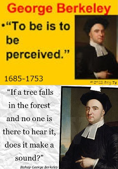
$\fbox{Note 2.3}$ The above is associated with Berkley's words:
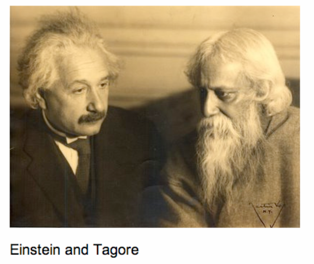
which is peculiar to dualism: This is opposite to Einstein's saying (i.e., monism proposition):
$(\sharp_1)$:
[The linguistic world view]:
To be is to be perceived
(by George Berkeley(1685-1753))
in Einstein and Tagore's conversation.
Since the Copenhagen interpretation ( due to Bohr, etc.) asserts that "measurement" is indispensable,
it is a matter of course that Einstein did not agree to the Copenhagen interpretation.
$(\sharp_2)$:
[The realistic world view]:
The moon is there whether one looks at it or not (= Physics holds without observers)
Example 2.21 [The resolution of the identity $I$; The word's partition]
Let $[C_0(\Omega ) \subseteq L^\infty (\Omega, \nu ) \subseteq B(L^2 (\Omega, \nu ))]$ be the classical basic structure. We find the similarity between an observable ${\mathsf O}$ and the resolution of the identity $I$ in what follows. Consider an observable ${\mathsf O} \equiv$ $({}X , {\cal F} , F{}) $ in ${L^\infty (\Omega)}$ such that $X$ is a countable set (i.e., $X \equiv \{ x_1, x_2, ... \}$) and ${\cal F}={\cal P}(X) = \{ \Xi \;|\;\Xi \subseteq X \}$, i.e., the power set of $X$. Then, it is clear that
| (i): | $F(\{ x_k \}) \ge 0$ for all $k=1,2,...$ |
| (ii): | $\sum_{k=1}^{\infty} [F(\{ x_k \})](\omega ) = 1$ $\quad (\forall \omega \in \Omega )$, |
which imply that the $[{}F({}\{ x_k \}{}) \;{}: \; k=1,2,...{}]$ can be regarded as the resolution of the identity element $I$. Thus we say that
| $\bullet$ | An observable ${\mathsf O}$ $\big(\equiv$ $({}X , {\cal F} , F{}) \big)$ in ${L^\infty (\Omega)}$ can be regarded as \begin{align*} \mbox{ " the resolution of the identity $I$" } \end{align*} |
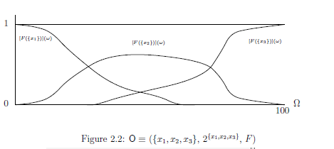
In Figure 2.2, assume that $\Omega=[0,100]$ is the axis of temperatures (°C), and put $X=\{ \mbox{C(="cold")}$, $\mbox{L}$ $\mbox{(="lukewarm"}$ $=\mbox{"not hot}$ $\mbox{enough")}$, $\mbox{H(="hot") }$ $\}$. And further, put $f_{x_1}=f_{\mbox{ C}}$, $f_{x_2}=f_{\mbox{ L}}$, $f_{x_3}=f_{\mbox{ H}}$. Then, the resolution $\{f_{x_1}, f_{x_2}, f_{x_3} \}$ can be regarded as the word's partition $ \mbox{C(="cold")}$, $\mbox{L(="lukewarm"="not hot}$ $\mbox{ enough")}$, $\mbox{H(="hot") }$. Also, putting
\begin{align*} {\cal F} (=2^X) =\{ \emptyset, \{x_1\},\{x_2\},\{x_3\}, \{x_1,x_2\},\{x_2,x_3\},\{x_1, x_3\}, X\} \end{align*} and \begin{align*} & [F(\emptyset )](\omega ) = 0, \;\; [F(X)](\omega)=f_{x_1}(\omega)+f_{x_2}(\omega)+f_{x_3}(\omega)=1 \\ & [F(\{x_1\})](\omega ) =f_{x_1}(\omega), \;\; [F(\{x_2\})](\omega ) =f_{x_2}(\omega), \;\; [F(\{x_3\})](\omega ) =f_{x_3}(\omega) \\ & [F(\{x_1,x_2\})](\omega ) =f_{x_1}(\omega)+f_{x_2}(\omega), \;\; [F(\{x_2,x_3 \})](\omega ) =f_{x_2}(\omega)+f_{x_3}(\omega) \\ & [F(\{x_1,x_3\})](\omega ) =f_{x_1}(\omega)+f_{x_3}(\omega) \end{align*}then, we have the observable $(X, {\cal F}(=2^X), F)$ in $L^\infty ([0,100])$.
Example 2.22 [Triangle observable]Let $[C_0(\Omega ) \subseteq L^\infty (\Omega, \nu ) \subseteq B(L^2 (\Omega, \nu ))]$ be the classical basic structure. For example, define the state space $\Omega$ by the closed interval $[0,100]$ $( \subseteq {\mathbb R})$. For each $n \in {\mathbb N}_{10}^{100} = \{0,10,20,\ldots,100\}$, define the (triangle) continuous function $g_{n}:\Omega \to {\mathbb R}$ by
\begin{align} g_{n} (\omega) = \left\{\begin{array}{ll} 0 & \quad (0 {{\; \leqq \;}}\omega {{\; \leqq \;}}n-10 ) \\ {\displaystyle \frac{\omega - n -10}{10} } & \quad (n-10 {{\; \leqq \;}}\omega {{\; \leqq \;}}n ) \\ {\displaystyle - \frac{\omega - n + 10}{10} } & \quad (n {{\; \leqq \;}}\omega {{\; \leqq \;}}n+10 ) \\ 0 & \quad (n+10 {{\; \leqq \;}}\omega {{\; \leqq \;}}100 ) \end{array}\right. \tag{2.57} \end{align}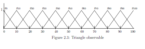
Putting $Y={\mathbb N}_{10}^{100}$ and define the triangle observable ${\mathsf O}^{\triangle}= (Y , 2^Y, F^{\triangle} )$ such that
\begin{align*} & [F^{\triangle}(\emptyset )](\omega ) = 0, \qquad [F^{\triangle}(Y )](\omega ) = 1 \\ & [F^{\triangle} (\Gamma )](\omega ) = \sum\limits_{n \in \Gamma } g_n (\omega ) \quad (\forall \Gamma \in 2^{{\mathbb N}_{10}^{100} }) \end{align*}Then, we have the triangle observable ${\mathsf O}^{\triangle}= (Y (= {{\mathbb N}_{10}^{100} } ), 2^Y, F^{\triangle} )$ in $L^\infty ([0,100])$.
Example 2.23 [Normal observable ( or, Gauss observable )]
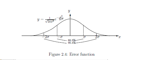

Consider a classical basic structure $[C_0(\Omega ) \subseteq L^\infty (\Omega, \nu ) \subseteq B(L^2 (\Omega, \nu ))]$. Here, $\Omega = {\mathbb R}(=\mbox{the real line})$ or, $\Omega = \mbox{interval }[a, b{}] $ $\;(\subseteq {\mathbb R} )$, which is assumed to have Lebesgue measure $\nu (d\omega) (= d \omega )$. Let $\sigma>0$, which is call a standard deviation. The normal observable ${\mathsf O}_{G_\sigma} {{=}} ({\mathbb R}, {\cal B}_{\mathbb R}, G_{\sigma})$ in $L^\infty (\Omega,\nu)$ is defined by
\begin{align*} [G_{\sigma}(\Xi)] (\omega) = \frac{1}{\sqrt{2 \pi \sigma^2}} \int_{\Xi} e^{- \frac{(x - \omega)^2}{2 \sigma^2}} dx \quad (\forall \Xi \in {\cal B}_{\mathbb R}(\mbox{Borel field}), \forall \omega \in \Omega (={\mathbb R} \mbox{ or } [a,b] )) \end{align*} This is the most fundamental observable in statistics.The following examples introduced in Example 2.24 and Example 2.25 are not $C^*$- observables but $W^*$- observables. This implies that the $W^*$-algebraic approach is more powerful than the $C^*$-algebraic approach. Although the $C^*$-observable is easy, it is more narrow than the $W^*$- observable. Thus, throughout this note, we mainly devote ourselves to $W^*$-algebraic approach.
Example 2.24 [Exact observable]
Consider the classical basic structure: $[C_0(\Omega ) \subseteq L^\infty (\Omega, \nu ) \subseteq B(L^2 (\Omega, \nu ))]$. Let ${\mathcal B}_\Omega$ be the Borel field in $\Omega$, i.e., the smallest $\sigma$-field that contains all open sets. For each $\Xi \in {\cal B}_\Omega$, define the definition function $\chi_{{}_\Xi}: \Omega \to {\mathbb R}$ such that
\begin{align} \chi_{{}_\Xi} ({}\omega{}) = \left\{\begin{array}{ll} 1 & ( \omega \in \Xi) \\ \\ 0 & ( \omega \notin \Xi ) \quad \end{array}\right. \tag{2.58} \end{align}Put $[F^{{ (exa)}}(\Xi)](\omega)=\chi_\Xi(\omega)$ $(\Xi \in {\cal B}_\Omega , \omega \in \Omega )$. The triplet ${\mathsf O}^{{ (exa)}}= (\Omega, {\cal B}_\Omega , F^{{ (exa)}})$ is called the exact observable in $L^\infty (\Omega , \nu )$. This is the $W^*$-observable and not $C^*$-observable, since $[F^{{ (exa)}}(\Xi)](\omega)$ is not always continuous. For the argument about the sample probability space (cf. Definition 2.19), see Example 2.33.
Example 2.25 [Rounding observable] Define the state space $\Omega$ by $\Omega = [0,100]$. For each $n \in {\mathbb N}_{10}^{100} {{=}} \{0,10,20,\ldots,100\}$, define the discontinuous function $g_{n}:\Omega \to [0,1]$ such that
\begin{align*} g_{n} (\omega) = \left\{\begin{array}{ll} 0 & \quad (0 {{\; \leqq \;}}\omega {{\; \leqq \;}}n-5 ) \\ 1 & \quad (n-5 {{\; < \;}}\omega {{\; \leqq \;}}n +5) \\ 0 & \quad (n+5 {{\; < \;}}\omega {{\; \leqq \;}}100 ) \end{array}\right. \end{align*}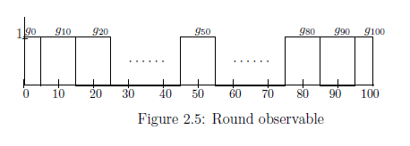
Define the observable ${\mathsf O}_{{RND}}= (Y ({{=}} {\mathbb N}_{10}^{100}) , 2^Y, G_{{RND}})$ in $L^\infty (\Omega , \nu )$ such that
\begin{align*} & [G_{{RND}}(\emptyset )](\omega ) = 0, \quad [G_{{RND}}(Y )](\omega ) = 1 \\ & [G_{{RND}} (\Gamma )](\omega ) = \sum\limits_{n \in \Gamma } g_n (\omega ) \quad (\forall \Gamma \in 2^Y = 2^{{\mathbb N}_{10}^{100} }) \end{align*}Recall that $g_n$ is not continuous. Thus, this is not $C^*$-observable but $W^*$-observable.
