Therefore, if \( \Omega \) is compact, the condition \( \lim_{\omega \to \infty} f(\omega)=0 \) is not needed, and thus, $C_0(\Omega)$ is usually denoted by $C(\Omega)$. In this note, even if $\Omega$ is compact, we often denote $C(\Omega)$ by $C_0(\Omega)$.
Defining the norm $\| \cdot \|_{C_0(\Omega )}$ in a complex vector space $C_0(\Omega)$ such that
2.3.1 Classical basic structure$[C_0(\Omega ) \subseteq L^\infty (\Omega, \nu ) \subseteq {B(L^2( \Omega, \nu ))}]$
In classical systems, the basic structure$[{\mathcal A} \subseteq \overline{\mathcal A} \subseteq B(H)]$ is restricted to the classical basic structure:
\begin{align*}
[C_0(\Omega ) \subseteq L^\infty (\Omega, \nu )
\subseteq {B(L^2( \Omega, \nu ))}]
\end{align*}
And we get the following diagram:
In what follows, we shall explain this diagram.
2.3.1.1 Commutative $C^*$-algebra $C_0(\Omega)$
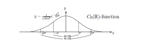
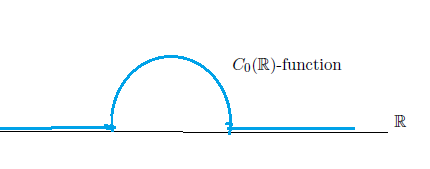
Let $\Omega$ a locally compact space, for example, it suffices to image $\Omega$ as follows.
\begin{align*}
&
{\mathbb R}(=\mbox{the real line}), \;\;{\mathbb R}^2(=\mbox{plane}), \;\;
{\mathbb R}^n(=\mbox{$n$-dimensional Euclidean space}), \;\;
\\
\\
&
[a, b ](=\mbox{interval}), \;\;
\underset{\mbox{ (with discrete metric $d_D$)}}{\mbox{finite set}\Omega(=\{\omega_1,..., \omega_n\})}
\end{align*}
where the discrete metric $d_D$ is defined by
\[
d_D(\omega, \omega')=1 \;(\omega \not= \omega'),
=0\;(\omega = \omega')
\]
Define the continuous functions space $C_0(\Omega)$ such that
\begin{align}
C_0(\Omega)
=
\{f:\Omega \to {\mathbb C} \;|\;
\mbox{$f$ is complex-valued continuous on $\Omega$, }\lim_{\omega \to \infty} f(\omega)=0 \}
\end{align}
where "$\lim_{\omega \to \infty} f(\omega)=0$" means
(A1): for any positive real $\epsilon >0$, there exists a compact set
$K (\subseteq \Omega)$ such that
\begin{align*}
\{ \omega \;|\; \omega \in \Omega \setminus K, |f(\omega)| > \epsilon \}
=
\emptyset
\end{align*}
For example,
Let $\Omega$ be a locally compact space, and consider the $\sigma$-finite measure space $(\Omega, {\cal B}_{\Omega}, \nu)$, where, ${\cal B}_{\Omega}$ is the Borel field, i.e., the smallest $\sigma$-field that contains all open sets. Further, assume that
| (A1): | for any open set $U \subseteq \Omega$, it holds that $0 < \nu (U) {\; \leqq \;} \infty$ |
| $\fbox{Note 2.1}$ | Without loss of generality, we can assume that $\Omega$ is compact by the Stone-Cech compactification. Also, we can assume that $\nu(\Omega)=1$. |
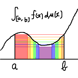
Define the Banach space $L^r (\Omega, \nu)$ (where, $r = 1, 2, \infty $) by the all complex-valued measurable functions $f: \Omega\to {\mathbb C}$ such that
\begin{align} \|f\|_{L^r (\Omega, \nu)} < \infty \end{align} The norm $\|f\|_{L^r (\Omega, \nu)} $ is defined by \begin{align} \|f\|_{L^r (\Omega, \nu)} = \left\{\begin{array}{ll} {\Big[ \int_{\Omega} |f (\omega)|^r \, \nu(d \omega) \Big]^{1/r}} \quad & \mbox{(when $r = 1, 2$)} \\ \\ \underset{\omega \in \Omega}{\mbox{ ess.sup} }|f (\omega)| & \mbox{(when $r = \infty$)} \end{array}\right. \end{align} where \begin{align*} \mbox{ ess.sup}_{\omega \in \Omega} |f (\omega)| = \sup \{ a \in {\mathbb R} \;|\; \nu(\{ \omega \in \Omega \; :\; |f (\omega)| {\; \geqq \;}a \; \}) >0 \} \end{align*}$L^r (\Omega, \nu)$ is often denoted by $L^r (\Omega)$ or $L^r (\Omega, {\cal B}_{\Omega}, \nu)$.
Therefore, for any $F \in C_0(\Omega)$, $\rho \in C_0(\Omega)^*={\mathcal M}(\Omega)$, we have the bi-linear form which is written by the several ways such as
\begin{align} \rho(F) = {}_{\stackrel{{}}{C_0(\Omega)^* }}\Big(\rho, F \Big){}_{\stackrel{{}}{{ C_0(\Omega) } }} = {}_{\stackrel{{}}{{\mathcal M}(\Omega)}}\Big(\rho, F \Big){}_{\stackrel{{}}{{ C_0(\Omega) } }} = \int_\Omega F(\omega) \rho( d \omega ) \tag{2.36} \end{align} Also, the dual norm is calculated as follows. \begin{align} & \|\rho\|_{C_0(\Omega)^* } = \sup \{ |\rho(F) \;|\; \|F\|_{C_0(\Omega)}=1 \} = \sup_{||F||_{C_0(\Omega)}=1}| \int_\Omega F(\omega ) \rho(d\omega)| \nonumber \\ = & \sup_{\Xi, \Gamma \in {\mathcal B}_\Omega} \Big( |Re(\rho(\Xi))-Re(\rho(\Xi^c))|^2 + |Im(\rho(\Gamma))-Im(\rho(\Gamma^c))|^2 \Big)^{1/2} \nonumber \\ = & \|\rho\|_{{\mathcal M}(\Omega)} \tag{2.37} \end{align}where, $\Xi^c$ is the complement of $\Xi$, and $Re(z)$="the real part of the complex number $z$", $Im(z)$="the imaginary part of the complex number $z$".
2.3.1.2 Commutative $W^*$-algebra $L^\infty (\Omega, \nu)$
Further, we see that \begin{align*} L^1(\Omega, \nu )^* = L^\infty (\Omega , \nu ) \qquad \mbox{ in the same sense, } \qquad L^1(\Omega, \nu ) = L^\infty (\Omega , \nu )_* \end{align*} Also, }it is clear that \begin{align*} C_0(\Omega ) \subseteq L^\infty (\Omega, \nu ) \end{align*}For any $f \in L^\infty (\Omega, \nu )$, there exist $f_n \in C_0(\Omega), n=1,2,.. $ such that
\begin{align*} \left\{\begin{array}{ll} \nu(\{ \omega \in \Omega \;|\; \lim_{n \to \infty } f_n (\omega ) \not= f(\omega) \}=0 \\ \\ |f_n (\omega )|\le \|f \|_{L^\infty (\Omega, \nu )} \quad (\forall \omega \in \Omega, \forall n=1,2,3,... ) \end{array}\right. \end{align*}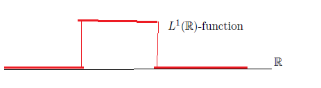
2.3.2 Classical basic structure$[C_0(\Omega ) \subseteq L^\infty (\Omega, \nu ) \subseteq {B(L^2( \Omega, \nu ))}]$ and State space
Consider the classical basic structure $[C_0(\Omega ) \subseteq L^\infty (\Omega, \nu ) \subseteq {B(L^2( \Omega, \nu ))}]$. Then, we see the following diagram:Remark 2.13 [The case that $\Omega$ is finite: $C_0(\Omega)=L^\infty(\Omega,\nu)$, ${\mathcal M}(\Omega ) = L^1(\Omega, \nu )$] Let $\Omega$ be a finite set $\{\omega_1,\omega_2,...,\omega_n \}$ with the discrete metric $d_D$ and the counting measure $\nu$. Here, the counting measure $\nu$ is defined by
\[ \nu( D )= \sharp [D] (= \mbox{"the number of the elements of $D$"} ) \] Then, we see that \[ C_0(\Omega ) = \{ F : \Omega \to {\mathbb C} \;|\; \mbox{ $F$ is a complex valued function on $\Omega$} \} = L^\infty (\Omega, \nu ) \] And thus, we see that \[ \rho \in {\mathcal M}_{+1}(\Omega ) \;\; \Longleftrightarrow \;\; \rho = \sum_{k=1}^n p_k \delta_{\omega_k } \;\;( \sum_{k=1}^n p_k=1, p_k \ge 0) \] and \[ f \in L^1_{+1}(\Omega, \nu ) \;\; \Longleftrightarrow \;\; \sum_{k=1}^n f(\omega_k ) =1. \;\; f(\omega_k )\ge 0 \] In this sense, we have the following identifications: \[ {\mathcal M}_{+1}(\Omega ) = L^1_{+1}(\Omega, \nu ) \quad (\mbox{ or, } {\mathcal M}(\Omega ) = L^1 (\Omega, \nu ) ) \] After all, we have the following identification: \[ C_0(\Omega )= L^\infty(\Omega) = {\mathbb C}^n \qquad {\mathcal M}(\Omega )= L^1(\Omega) = {\mathbb C}^n \tag{2.44} \] where the norm $\| \cdot \|_{C_0(\Omega )}$ in the former is defined by \begin{align} \| z \|_{C_0(\Omega )}= \max_{k=1,2,...,n} |z_k | \qquad \forall z= \left[\begin{array}{l} z_1 \\ z_2 \\ \vdots \\ x_n \end{array}\right] \in {\mathbb C}^n \tag{2.45} \end{align} and the norm $\| \cdot \|_{{\mathcal M}(\Omega )}$ in the latter is defined by \begin{align} \| z \|_{{\mathcal M}(\Omega )}= \sum_{k=1}^n |z_k | \qquad \forall z= \left[\begin{array}{l} z_1 \\ z_2 \\ \vdots \\ x_n \end{array}\right] \in {\mathbb C}^n \tag{2.46} \end{align}