In quantum system, the basic structure$[{\mathcal A} \subseteq \overline{\mathcal A} \subseteq B(H)]$ is characterized as
Before we explain "compact operators class ${\mathcal C}(H)$" and "trace class ${\mathcal Tr}(H)$" in Theorem 2.6 and 2.7, we have to prepare "Dirac notation" and "CONS" as follows.
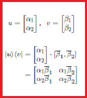
Let $H$ be a Hilbert space. For any $u, v \in H$, define $| u \rangle \langle v | \in B(H)$ such that
Here, $\langle v |$ $\big[$ resp. $| u \rangle$ $\big]$ is called the "Bra-vector" $\big[$ resp. "Ket-vector"$\big]$.
In addition, an ONS $\{e_k\}_{k=1}^\infty$ is called a complete orthonormal system (i.e., CONS), if it satisfies
2.2.1: Quantum basic structure$[{\mathcal C}(H) \subseteq B(H) \subseteq B(H)]$: Compact operator, Trace operator
where "compact operators class ${\mathcal C}(H)$" and "trace class ${\mathcal Tr}(H)$"
 Definition 2.5 [(i): Dirac notation]
 [(ii):ONS(orthonormal system), CONS(complete orthonormal system)]
The sequence $\{e_k\}_{k=1}^\infty$ in a Hilbert space $H$ is called an orthonormal system (i.e., ONS), if it satisfies
[(ii):ONS(orthonormal system), CONS(complete orthonormal system)]
The sequence $\{e_k\}_{k=1}^\infty$ in a Hilbert space $H$ is called an orthonormal system (i.e., ONS), if it satisfies
$(\sharp)$ $\langle e_k, e_j \rangle = \left\{\begin{array}{ll}
1 \quad & (k = j )
\\
0 \quad & (k \not= j )
\end{array}\right.
$
$(\sharp)$ $\langle x, e_k \rangle =0
\;
(\forall k=1,2,...)$ implies that $x=0$.
Let ${\mathcal C}(H) (\subseteq B(H))$
be the compact operators class.
Then, we see the following (C$_1$)-(C$_4$) $\Big($ particularly, "(C$_1$)$\leftrightarrow$ (C$_2$)" may be regarded as the definition of the compact operators class ${\mathcal C}(H) (\subseteq B(H))$ $\Big)$.

$(C_1)$: $T \in {\mathcal C}(H)$.That is,
$(C_2)$: There exist two ONSs $\{e_k\}_{k=1}^\infty$ and $\{f_k\}_{k=1}^\infty$ in the Hilbert space $H$ and a positive real sequence $\{\lambda_k \}_{k=1}^\infty$ (where, $\lim_{k \to \infty } \lambda_k =0$ ) such that
\begin{align}
T=\sum_{k=1}^\infty \lambda_k |e_k \rangle \langle f_k|
\qquad
(\mbox{in the sense of weak topology})
\tag{2.10}
\end{align}
$(C_3)$: ${\mathcal C}(H)( \subseteq B(H))$ is a $C^*$-algebra. When $T (\in {\mathcal C}(H))$ is represented as in (C$_2$), the following equality holds
\begin{align}
\| T \|_{B(H)}= \max_{k=1,2, \cdots } \lambda_k
\tag{2.11}
\end{align}
$(C_4)$: The weak closure of ${\mathcal C}(H)$ is equal to $B(H)$. That is,
\begin{align}
\overline{{\mathcal C}(H)}=B(H)
\label{2.12}
\end{align}
 Theorem 2.7 [The properties of trace class ${\mathcal Tr}(H)$]
Let ${\mathcal Tr}(H) (\subseteq B(H))$ be the trace class. Then, we see the following (D$_1$)-(D$_4$)( particularly, "(D$_1$)$\leftrightarrow$ (D$_2$)" may be regarded as the definition of the trace class ${\mathcal Tr}(H) (\subseteq B(H))$).
$(D1)$: $T \in {\mathcal Tr}(H) (\subseteq {\mathcal C}(H) \subseteq B(H))$.
$(D2)$: There exist two ONSs $\{e_k\}_{k=1}^\infty$ and $\{ f_k \}_{ k=1}^\infty$ in the Hilbert space $H$ and a positive real sequence $\{\lambda_k \}_{k=1}^\infty$ (where,
$\sum_{k=1}^{ \infty } \lambda_k < \infty$) such that
\begin{align*}
T=\sum_{k=1}^\infty \lambda_k |e_k \rangle \langle f_k|
\qquad
(\mbox{in the sense of weak topology})
\end{align*}
$(D3)$: It holds that
\begin{align}
{\mathcal C}(H)^*={\mathcal Tr}(H)
\tag{2.13}
\end{align}
Here, the dual norm $\| \cdot \|_{{\mathcal C}(H)^*}$ is characterized as the trace norm $\| \cdot \|_{Tr}$ such as
\begin{align}
\|T\|_{Tr}= \sum_{k=1}^\infty \lambda_k
\tag{2.14}
\end{align}
when $T (\in {\mathcal Tr}(H))$ is represented as in (D$_2$),
$(D4)$: Also, it holds that
\begin{align}
{\mathcal Tr}(H)^*=B(H)
\qquad
\mbox{in the same sense,}
\qquad
{\mathcal Tr}(H)=B(H)_*
\label{2.15}
\end{align}
2.2.2 Quantum basic structure$[{\mathcal C}(H) \subseteq B(H) \subseteq B(H)]$ and State space
Consider the quantum basic structure:
\begin{align}
[{\mathcal C}(H) \subseteq B(H) \subseteq B(H)]
\end{align}
and see the following diagram:
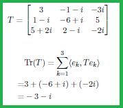 Definition 2.9 [Tr: trace].
Define the trace ${\mbox{Tr}}: {\mathcal Tr}(H) \to {\mathbb C}$ such that
\begin{align}
{\mbox{Tr}}(T)
=
\sum_{n=1}^\infty \langle e_n, T e_n \rangle
\qquad (\forall T \in {\mathcal Tr}(H) )
\end{align}
where $\{e_n\}_{n=1}^\infty $ is a CONS in $H$. It is well known that
the ${\mbox{Tr}}(T)$ does not depend on the choice of CONS $\{e_n\}_{n=1}^\infty $.
Thus, clearly we see that
\begin{align}
{}_{{}_{{\mathcal Tr}{H}}}\Big(
|u \rangle \langle u |,
F
\Big){}_{{}_{B(H)}}
=
{\mbox{Tr}}
(
|u \rangle \langle u |
\cdot
F
)
=
\langle u, F u \rangle
\quad
(\forall ||u||_H=1, F \in B(H)
)
\end{align}
Definition 2.9 [Tr: trace].
Define the trace ${\mbox{Tr}}: {\mathcal Tr}(H) \to {\mathbb C}$ such that
\begin{align}
{\mbox{Tr}}(T)
=
\sum_{n=1}^\infty \langle e_n, T e_n \rangle
\qquad (\forall T \in {\mathcal Tr}(H) )
\end{align}
where $\{e_n\}_{n=1}^\infty $ is a CONS in $H$. It is well known that
the ${\mbox{Tr}}(T)$ does not depend on the choice of CONS $\{e_n\}_{n=1}^\infty $.
Thus, clearly we see that
\begin{align}
{}_{{}_{{\mathcal Tr}{H}}}\Big(
|u \rangle \langle u |,
F
\Big){}_{{}_{B(H)}}
=
{\mbox{Tr}}
(
|u \rangle \langle u |
\cdot
F
)
=
\langle u, F u \rangle
\quad
(\forall ||u||_H=1, F \in B(H)
)
\end{align}
2.2: Quantum basic structure $[{\mathcal C}(H) \subseteq$ $ B(H) \subseteq B(H)]$
This web-site is the html version of "Linguistic Copehagen interpretation of quantum mechanics; Quantum language [Ver. 4]" (by Shiro Ishikawa; [home page] )
PDF download : KSTS/RR-18/002 (Research Report in Dept. Math, Keio Univ. 2018, 464 pages)
Contents:
Theorem 2.6 [The properties of compact operators class ${\mathcal C}(H)$]
