18.1: Reliability in psychological tests
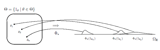
In this section, let us consider the reliability of the psychological tests for a group of students. We introduce the examples which is a measurement theoretical characterization of the tests which measure the mathematical intelligences of students. Let $\Theta := \{\theta_1,\theta_2,\dots,\theta_n\}$ be a set of students, say, there are $n$ students $\theta_1,\theta_2,\dots,\theta_n$. Define the counting measure $\nu_c$ on $\Theta$ such that $\nu_c(\{\theta_i\}) = 1$ ($i=1,2,\dots,n$). The $\Theta$ will be regarded as the state. For each $\theta_i \;(\in \Theta)$, we define $1_{\theta_i} \;(\in L_{+1}^1(\Theta,\nu_c))$ by $1_{\theta_i}(\theta) = 1 \;(\mbox{if } \theta = \theta_i), \;\; = 0 \;(\mbox{if }\theta \ne \theta_i)$. Recall that $\Theta$ can be identified with the $\{1_{\theta_i} \;|\; \theta_i \in \Theta\}$ under the identification: $\Theta \ni \theta_i \leftrightarrow 1_{\theta_i} \in \{1_\theta \;|\; \theta \in \Theta\}$. For simplicity, we will start with the test for one student $\theta_i \;(\in \Theta)$. Let $(\Omega_{\mathbb R},{\cal F}_{\Omega_{\mathbb R}},d\omega)$ be the Lebesgue measure space where $\Omega_{\mathbb R} = {\mathbb R}$.

Example 18.1 (Mathematics test for a student $\theta_i$)
Let $\Theta := \{\theta_1,\theta_2,\dots,\theta_n\}$ be a state space which is identified with the set of the students. The mathematical intelligence of the student $\theta_i \;(\in \Theta)$ is assumed to be represented by a statistical state $\Phi_\ast(1_{\theta_i}) \;(\in L_{+1}^1(\Omega_{\mathbb R},d\omega))$ ($i=1,2,\dots,n$) where $\Phi_\ast : L^1(\Theta,\nu_c) \to L^1(\Omega_{\mathbb R},d\omega)$ is a pre-dual Markov causal operator of $\Phi : L^\infty(\Omega_{\mathbb R},d\omega) \to L^\infty(\Theta,\nu_c)$.
Let ${\mathsf O} := (X_{\mathbb R},{\cal F}_{X_{\mathbb R}},F)$ be an observable in $L^\infty(\Omega_{\mathbb R},d\omega)$. Axiom${}^{{ (m)}}$ 1($\S$9.1) asserts that
| $(A):$ | the probability that the score (measured value) of the student $\theta_i \;(\in \Theta)$ obtained by the statistical measurement ${\mathsf M}_{L^\infty(\Omega_{\mathbb R},d\omega)}({\mathsf O}, S_{[\ast]}(\Phi_\ast(1_{\theta_i})))$ belongs to a set $\Xi \;(\in {\cal F}_{X_{\mathbb R}})$ is given by $$ {}_{L^1(\Omega_{\mathbb R},d\omega)} \langle {\Phi_\ast(1_{\theta_i})}, {F(\Xi)} \rangle_{L^\infty(\Omega_{\mathbb R},d\omega)} \; \Big(= \int_{\Omega_{\mathbb R}} [F(\Xi)](\omega) \, [\Phi_\ast(1_{\theta_i})](\omega) \, d\omega\Big). $$ |
Remark 18.2 In the above, readers may have the question such that
| $(B):$ | What is the unknown pure state $[\ast]$ in $S_{[\ast]}$? |
Imaging the deterministic causal map $\psi: \Theta \to \Omega_{\mathbb R} $, we may consider that $$ [\ast]= \psi (\theta_i) = \int_{\Omega_{\mathbb R}} \omega [\Phi_\ast(1_{\theta_i})](\omega) \, d\omega $$ Also, note that the $[\ast]$ does not play an important role in this chapter since Bayes's theorem 9.11 is not used.
Remark 18.3 It should be kept in mind that the variance $\sigma_i^2$ of the intelligence of $\theta_i \;(\in \Theta)$ ($i=1,2,\dots,n$) is not constant, that is to say, we do not assume that $\sigma_i^2 = \sigma_j^2$ ($\forall i, \forall j$):
\begin{align} \sigma_i^2 := \int_{\Omega_{\mathbb R}} (\omega-\mu_i)^2 \, [\Phi_\ast(1_{\theta_i})](\omega) \, d\omega \quad (i=1,2,\dots,n), \tag{18.1} \end{align} where $\mu_i$ is an expectation of $\Phi_\ast(1_{\theta_i})$: \begin{align} \mu_i := \int_{\Omega_{\mathbb R}} \omega \, [\Phi_\ast(1_{\theta_i})](\omega) \, d\omega \quad (i=1,2,\dots,n). \tag{18.2} \end{align}18.1.2: Group measurement (= parallel measurement)

The above example is the test for a student $\theta_i \;(\in \Theta)$. $\quad$ Keeping this in mind, we will next consider the test for a group of $n$ students. Let $ \Omega_{\mathbb R}^n={\mathbb R}^n $, and let $(\Omega_{\mathbb R}^n,{\cal F}_{\Omega_{\mathbb R}^n},d\omega^n)$ be a $n$-dimensional Lebesgue measure space. $\quad \quad $ Furthermore, let ${\mathsf O} := (X_{\mathbb R},{\cal F}_{X_{\mathbb R}},F)$ and ${\mathsf M}_{L^\infty(\Omega_{\mathbb R},d\omega)}({\mathsf O},$ $ S_{[\ast]}(\Phi_\ast(1_{\theta_i})))$ ($i=1,2,\dots,n$) be as in above example. Here, we consider a parallel measurement ${\mathsf M}_{L^\infty(\Omega_{\mathbb R}^n,d\omega^n)} (\widehat{\mathsf O}, S_{[\ast]}(\widehat{\rho}))$ where $\widehat{\mathsf O} := (X_{\mathbb R}^n,{\cal F}_{X_{\mathbb R}^n},\widehat{F})$ is an observable in $L^\infty(\Omega_{\mathbb R}^n,d\omega^n)$. If
\begin{align} [\widehat F (\Xi_1 \times \Xi_2 \times \cdots \times \Xi_n)](\omega_1,\omega_2,\dots,\omega_n) = [F(\Xi_1)](\omega_1) \cdot [F(\Xi_2)](\omega_2) \cdots [F(\Xi_n)](\omega_n), \end{align} and \begin{align} \widehat{\rho} (\omega_1,\omega_2,\dots,\omega_n) = [\Phi_\ast(1_{\theta_1})](\omega_1) \cdot [\Phi_\ast(1_{\theta_2})](\omega_2) \cdots [\Phi_\ast(1_{\theta_n})](\omega_n), \end{align}then, the parallel measurement ${\mathsf M}_{L^\infty(\Omega_{\mathbb R}^n,d\omega^n)} (\widehat{\mathsf O}, S_{[\ast]}(\widehat \rho))$ is denoted by
$$ \otimes_{\theta_i \in \Theta} {\mathsf M}_{L^\infty(\Omega_{\mathbb R},d\omega)}({\mathsf O}, S_{[\ast]}(\Phi_\ast(1_{\theta_i}))). $$In addition, we introduce the following notations concerning tensor product:
\begin{align} \otimes_{k=1}^n L^\infty(\Omega_{\mathbb R},d\omega) = L^\infty(\Omega_{\mathbb R}^n,d\omega^n) \quad \mbox{and} \quad \otimes_{k=1}^n L^1(\Omega_{\mathbb R},d\omega) = L^1(\Omega_{\mathbb R}^n ,d\omega^n). \end{align} By the way, we introduce the test observable.Definition 18.4 [Test observable] The ${\mathsf O}_\tau = (X_{\mathbb R}, {\cal F}_{X_{\mathbb R}}, F_\tau)$ is called a { test observable} in $L^\infty (\Omega_{\mathbb R},d\omega)$, if $F_\tau$ satisfies the following no-bias condition:
\begin{align} \int_{X_{\mathbb R}} x \, [F_\tau(dx)](\omega) = \omega \quad (\forall \omega \in \Omega_{\mathbb R}). \tag{18.3} \end{align}Recall that the normal observable (cf. Example 2.23 ) and the exact observable (cf. Example 2.24 ).
For each $\theta_i \;(\in \Theta)$, we use the notation ${\mathsf M}_{{\mathsf O}_\tau}^{(i)}$ to the test for $\theta_i \;(\in \Theta)$ (the measurement of the test observable ${\mathsf O}_\tau$ for the statistical state $\Phi_\ast(1_{\theta_i})$):
\begin{align} {\mathsf M}_{{\mathsf O}_\tau}^{(i)} := {\mathsf M}_{L^\infty(\Omega_{\mathbb R},d\omega)}({\mathsf O}_\tau, S_{[\ast]}(\Phi_\ast(1_{\theta_i}))). \tag{18.4} \end{align}Now we are ready to consider the test for a set of the $n$ students in our measurement theory.
Definition 18.5 [Test, Group test] Let $\Theta := \{\theta_1,\theta_2,\dots,\theta_n\}$, $X_{\mathbb R} = \Omega_{\mathbb R} = {\mathbb R}$ and $\Phi_\ast : L_{+1}^1(\Theta,\nu_c) \to L_{+1}^1(\Omega_{\mathbb R},d\omega)$ be as in Example 18.1. Let ${\mathsf O}_\tau := (X_{\mathbb R},{\cal F}_{X_{\mathbb R}},F_\tau)$ be a test observable in $L^\infty(\Omega_{\mathbb R},d\omega)$. The measurement ${\mathsf M}_{L^\infty(\Omega_{\mathbb R},d\omega)}({\mathsf O}_\tau, S_{[\ast]}(\Phi_\ast(1_{\theta_i})))$ is called a { test for a student $\theta_i \;(\in \Theta)$} and symbolized by ${\mathsf M}_{{\mathsf O}_\tau}^{(i)}$ for short. And the measurement
\begin{align} \otimes_{\theta_i \in \Theta} {\mathsf M}_{L^\infty(\Omega_{\mathbb R},d\omega)}({\mathsf O}_\tau, S_{[\ast]}(\Phi_\ast(1_{\theta_i}))) \quad (\mbox{or in short, $\otimes_{\theta_i \in \Theta} {\mathsf M}_{{\mathsf O}_\tau}^{(i)}$}), \tag{18.5} \end{align} is called a { group test} and symbolized by ${\mathsf M}_{{\mathsf O}_\tau}^\otimes$ for short.| $(C):$ | $\;$ the probability that the score $\;\; (x_1,x_2,\dots,x_n) \;\; (\in X_{\mathbb R}^n)$ $\;\;$ obtained by the group test $\otimes_{\theta_i \in \Theta} {\mathsf M}_{L^\infty(\Omega_{\mathbb R},d\omega)}$ $({\mathsf O}_\tau, S_{[\ast]}(\Phi_\ast(1_{\theta_i})))$ (or in short, ${\mathsf M}_{{\mathsf O}_\tau}^\otimes$) belongs to the set $\times_{i=1}^n \Xi_i \;(\in {\cal F}_{X_{\mathbb R}^n})$ is given by \begin{align} \times_{\theta_i \in \Theta} {}_{L^1(\Omega_{\mathbb R},d\omega)} \langle {\Phi_\ast(1_{\theta_i})}, {F(\Xi)} \rangle_{L^\infty(\Omega_{\mathbb R},d\omega)} =: {\widehat P}_1(\times_{i=1}^n \Xi_i) =\times_{i=1}^n P_i(\Xi_i) \Big). \tag{18.6} \end{align} |
Here, $(X_{\mathbb R}, {\cal F}_{X_{\mathbb R}}, P_i)$ is a sample probability space of ${\mathsf M}_{{\mathsf O}_\tau}^{(i)}$. Let $W: X_{\mathbb R}^n \to {\mathbb R}$ be a statistics (i.e., measurable function). Then, ${\cal E}_{{\mathsf M}_{{\mathsf O}_\tau}^\otimes}[W]$, the expectation of $W$, is defined by
$$ \mathcal{E}_{{\mathsf M}_{{\mathsf O}_\tau}^\otimes}[W] = \int_{X_{\mathbb R}} \cdots \int_{X_{\mathbb R}} W(x_1, x_2, \dots, x_n) \, {\widehat P}_1(dx_1 \, dx_2 \cdots dx_n). $$
Definition 18.6
Let ${\mathsf O}_\tau := (X_{\mathbb R},{\cal F}_{X_{\mathbb R}},F_\tau)$ be a test observable in $L^\infty(\Omega_{\mathbb R},d\omega)$
(i: Score of $\theta_i$)
Let ${\mathsf M}_{L^\infty(\Omega_{\mathbb R},d\omega)}({\mathsf O}_\tau, S_{[\ast]}(\Phi_\ast(1_{\theta_i})))$ (or in short, ${\mathsf M}_{{\mathsf O}_\tau}^{(i)}$) be a {test} for a student $\theta_i \;(\in \Theta)$.
Here, we consider the expectation of $x_i \;(\in X_{\mathbb R})$ and its variance.
| $(\sharp_1):$ | $\displaystyle { Av}[{\mathsf M}_{{\mathsf O}_\tau}^{(i)}] := {\cal E}_{{\mathsf M}_{{\mathsf O}_\tau}^{(i)}} [x_i]$, |
| $(\sharp_2):$ | $\displaystyle { Var}[{\mathsf M}_{{\mathsf O}_\tau}^{(i)}] := {\cal E}_{{\mathsf M}_{{\mathsf O}_\tau}^{(i)}} \Big[ (x_i-{ Av}[{\mathsf M}_{{\mathsf O}_\tau}^{(i)}])^2 \Big]$. |
(ii: Scores of $n$ students) Let $\otimes_{\theta_i \in \Theta} {\mathsf M}_{L^\infty(\Omega_{\mathbb R},d\omega)}({\mathsf O}_\tau, S_{[\ast]}(\Phi_\ast(1_{\theta_i})))$ (or in short, ${\mathsf M}_{{\mathsf O}_\tau}^\otimes$) be a {group test}. Here, we consider the expectation of $\frac1n (x_1+x_2+\cdots+x_n)$ and its variance.
| $(\sharp_1):$ | $\displaystyle { Av}[{ M}^{\otimes}_{{\mathsf O}_\tau}] := {\cal E}_{{\mathsf M}_{{\mathsf O}_\tau}^\otimes} \Big[\frac1n (x_1+x_2+\cdots+x_n)\Big]$, |
| $(\sharp_2):$ | $\displaystyle { Var}[{\mathsf M}_{{\mathsf O}_\tau}^\otimes] := {\cal E}_{{\mathsf M}_{{\mathsf O}_\tau}^\otimes} \Big[\frac1n \sum_{k=1}^n (x_k-{ Av}[{\mathsf M}_{{\mathsf O}_\tau}^{\otimes}])^2\Big]$. |
where ${\mathsf O}_E := (X_{\mathbb R},{\cal F}_{X_{\mathbb R}},E)$ is an exact observable in $L^\infty(\Omega_{\mathbb R},d\omega)$.
