Put
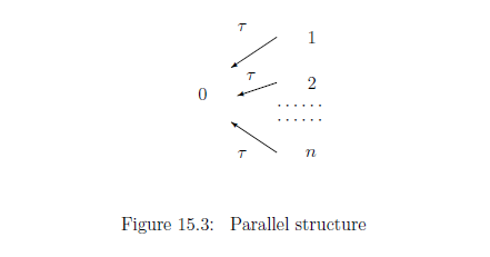
$T=\{ 0,1,2, \cdots, i , \cdots, n \}$,
which is the same as the tree (15.10),
that is,
15.4: Generalized linear model
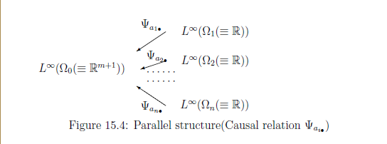
For each $i \in T$, define a locally compact space $\Omega_i$ such that
\begin{align} & \Omega_{0}={\mathbb R}^{m+1} = \Big\{ \beta =\begin{bmatrix} \beta_0 \\ \beta_1 \\ \vdots \\ \beta_m \end{bmatrix} \;:\; \beta_0, \beta_1, \cdots, \beta_m \in {\mathbb R} \Big\} \quad \tag{15.37} \\ & \Omega_{i}={\mathbb R} = \Big\{ \mu_i \;:\; \mu_i \in {\mathbb R} \Big\} \quad(i=1,2, \cdots, n ) \tag{15.38} \end{align} Assume that \begin{align} a_{ij} \in {\mathbb R} \qquad (i=1,2, \cdots, n, \;\;j=1,2, \cdots, m, (m+1 \le n) ) \tag{15.39} \end{align} which are called explanatory variables in the conventional statistics. Consider the deterministic causal map $\psi_{a_{i \tiny{\bullet}}}: \Omega_0(={\mathbb R}^{m+1}) \to \Omega_{i} (={\mathbb R})$ such that \begin{align} & \Omega_0={\mathbb R}^{m+1} \ni \beta =(\beta_0, \beta_1, \cdots, \beta_m ) \mapsto \psi_{a_{i \tiny{\bullet}}} ( \beta_0, \beta_1, \cdots, \beta_m ) = \beta_0 + \sum_{j=1}^m \beta_j a_{ij}= \mu_i \in \Omega_i ={\mathbb R} \\ & \qquad \qquad \qquad \qquad \qquad \qquad \qquad \qquad (i=1,2, \cdots, n) \tag{15.40} \end{align} Summing up, we see \begin{align} \beta= \begin{bmatrix} \beta_0 \\ \beta_1 \\ \beta_2 \\ \vdots \\ \beta_m \end{bmatrix} \mapsto \begin{bmatrix} \psi_{a_{1 \tiny{\bullet}}} ( \beta_0, \beta_1, \cdots, \beta_m) \\ \psi_{a_{2 \tiny{\bullet}}} ( \beta_0, \beta_1, \cdots, \beta_m) \\ \psi_{a_{3 \tiny{\bullet}}} ( \beta_0, \beta_1, \cdots, \beta_m) \\ \vdots \\ \psi_{a_{n \tiny{\bullet}}} ( \beta_0, \beta_1, \cdots, \beta_m) \end{bmatrix} = \begin{bmatrix} 1 & a_{1{1}} & a_{12} & \cdots & a_{1m} \\ 1 & a_{2{1}} & a_{22} & \cdots & a_{2m} \\ 1 & a_{3{1}} & a_{32} & \cdots & a_{3m} \\ 1 & a_{4{1}} & a_{42} & \cdots & a_{4m} \\ \vdots & \vdots & \vdots & \vdots & \vdots \\ 1 & a_{n{1}} & a_{n2} & \cdots & a_{nm} \end{bmatrix} \cdot \begin{bmatrix} \beta_0 \\ \beta_1 \\ \beta_2 \\ \vdots \\ \beta_m \end{bmatrix} \tag{15.41} \end{align}which is equivalent to the deterministic Markov operator $\Psi_{a_{i \tiny{\bullet} }}: L^\infty(\Omega_{i}) \to L^\infty(\Omega_0)$ such that
\begin{align} [{\Psi_{a_{i \tiny{\bullet} }}}(f_i)](\omega_0) = f_i( \psi_{a_{i \tiny{\bullet} }} (\omega_0)) \quad (\forall f_i \in L^\infty(\Omega_{i}), \;\; \forall \omega_0 \in \Omega_0, \forall i \in 1,2, \cdots, n) \tag{15.42} \end{align}Thus, under the identification: $\{a_{ij} \}_{j=1, \cdots, m} \Leftrightarrow \Psi_{a_{i \tiny{\bullet}}}$, the term "explanatory variable" means a kind of causality.
Therefore, we have the observable ${\mathsf O}_{0}^{a_{i \tiny{\bullet} }} {{\equiv}} ({\mathbb R}, {\cal B}_{{\mathbb R}}, \Psi_{a_{i \tiny{\bullet} }}G_{\sigma_{}})$ in $L^\infty (\Omega_{0}(\equiv {\mathbb R}^{m+1}))$ such that
\begin{align} & [\Psi_{a_{i \tiny{\bullet} }}(G_{\sigma_{}}(\Xi))] (\beta ) = [(G_{\sigma_{}}(\Xi))] (\psi_{a_{i \tiny{\bullet} }}(\beta )) = \frac{1}{(\sqrt{2 \pi \sigma_{}^2})} \underset{\Xi}{\int} \exp \Big[{- \frac{ (x - (\beta_0 + \sum_{j=1}^m a_{i{j}} \beta_j ))^2}{2 \sigma_{}^2}} \Big] dx \\ & \qquad \qquad (\forall \Xi \in {\cal B}_{{\mathbb R}}, \forall \beta =(\beta_0, \beta_1, \cdots, \beta_m )\in \Omega_{0} (\equiv {\mathbb R}^{m+1} )) \tag{15.43} \end{align}Hence, we have the simultaneous observable $\times_{i=1}^n{\mathsf O}_{0}^{a_{i \tiny{\bullet} }} {{\equiv}} ({\mathbb R}^n, {\cal B}_{{\mathbb R}^n}, \times_{i=1}^n \Psi_{a_{i \tiny{\bullet} }}G_{\sigma_{}})$ in $L^\infty (\Omega_{0}(\equiv {\mathbb R}^{m+1}))$ such that
\begin{align} & [(\times_{i=1}^n \Psi_{a_{i \tiny{\bullet} }}G_{\sigma_{}}) (\times_{i=1}^n \Xi_i)](\beta) = \times_{i=1}^n \Big( [\Psi_{a_{i \tiny{\bullet} }}G_{\sigma_{}}) (\Xi_i)](\beta)\Big) \nonumber \\ = & \frac{1}{(\sqrt{2 \pi \sigma_{}^2})^n} \underset{\times_{i=1}^n \Xi_i}{\int \cdots \int} \exp \Big[{- \frac{ \sum_{i=1}^n (x_i - (\beta_0 + \sum_{j=1}^ma_{i{j}} \beta_j ))^2}{2 \sigma_{}^2}} \Big] dx_1 \cdots dx_n \tag{15.44} \\ & \qquad \qquad (\forall \times_{i=1}^n \Xi_i \in {\cal B}_{{\mathbb R}^n}, \forall \beta =(\beta_0, \beta_1, \cdots, \beta_m ) \in \Omega_{0} (\equiv {\mathbb R}^{m+1} )) \nonumber \end{align} Assuming that $\sigma$ is variable, we have the observable ${\mathsf O}= \Big({\mathbb R}^n(=X) , {\mathcal B}_{{\mathbb R}^n}(={\mathcal F}), F \Big)$ in $L^\infty ( \Omega_0 \times {\mathbb R}_+ )$ such that \begin{align} & [F(\times_{i=1}^n \Xi_i )](\beta, \sigma_) = [(\times_{i=1}^n \Psi_{a_{i \tiny{\bullet} }}G_{\sigma_{}}) (\times_{i=1}^n \Xi_i)](\beta) \quad (\forall \times_{i=1}^n \Xi_i \in {\cal B}_{{\mathbb R}^n}, \forall (\beta , \sigma_{} ) \in {\mathbb R}^{m+1} (\equiv \Omega_0) \times {\mathbb R}_+ ) \\ & \tag{15.45} \end{align}Thus, we have the following problem.
Problem 15.8 [Generalized linear model in quantum language] Assume that a measured value $x=\begin{bmatrix} x_1 \\ x_2 \\ \vdots \\ x_n \end{bmatrix} \in X={\mathbb R}^n $ is obtained by the measurement ${\mathsf M}_{L^\infty(\Omega_{0} \times {\mathbb R}_+)}( {\mathsf O} \equiv (X, {\cal F}, F) , S_{[(\beta_0,\beta_1,\cdots, \beta_m , \sigma)]} {} )$. (The measured value is also called a response variable .) And assume that we do not know the state $ (\beta_0, \beta_1,\cdots, \beta_m, \sigma_{}^2 )$.
Then,
| $\quad$ | from the measured value $ x=( x_1, x_2, \ldots, x_n ) \in {\mathbb R}^{n}$, infer the $\beta_0, \beta_1, \cdots, \beta_m, \sigma_{}$! |
That is, represent the $(\beta_0, \beta_1, \cdots, \beta_m, \sigma_)$ by $(\hat{\beta}_0(x), \hat{\beta}_1(x),\cdots, \beta_m(x), \hat{\sigma}_{}(x))$ (i.e., the functions of $x$).
The answer is easy, since it is a slight generalization of Problem 15.3. However, note that the purpose of this chapter is to propose Problem 15.8 (i. e, the quantum linguistic formulation of the generalized linear model) and not to give the answer to Problem 15.8.
Remark 15.9 As a generalization of regression analysis, we also see measurement error model (cf. $\S$5.5 (117 page) in ref. [8] in $\S$0.0), That is, we have two different generalizations such as
\begin{align} \underset{\mbox{}}{\fbox{Regression analysis}} \xrightarrow[\mbox{{generalization}}]{} \left\{\begin{array}{ll} \mbox{①} : \underset{\mbox{}}{\fbox{generalized linear model}} \\ \mbox{②} \underset{\mbox{}}{\fbox{measurement error model}} \end{array}\right. \tag{15.46} \end{align} However, we believe that the ① is the main street.