11.6: "Whereof one cannot speak, thereof one must be silent"
This section is extracted from
In the conventional quantum mechanics,
the question:
"particle or wave?"
may frequently appear.
However, this is a foolish question.
On the other hand, the argument about the
"particle vs. wave"
is clear in quantum language.
As seen in the following table,
this argument is traditional:
11.6.1: "Particle or wave?" is a foolish question
$(\sharp):$
S. Ishikawa,
The double-slit quantum eraser experiments and Hardy's paradox in the quantum linguistic interpretation,
arxiv:1407.5143[quantum-ph],( 2014)
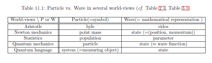
In the table 11.1, Newtonian mechanics (i.e., mass point $\leftrightarrow$ state) may be easiest to understand. Thus, "particle" and "wave" are not confrontation concepts.
Concerning "particle or wave", we have the following statements:
| $(A_1):$ | "Particle or wave" is a foolish question. |
| $(A_2):$ | Wheeler's delayed choice experiment is related to the question "particle or wave" |
| $(A_3):$ | How is Wheeler's delayed choice experiment described in terms of quantum mechanics? |
11.6.2: Preparation
Let us start from the review of $\S$2.10 (de Broglie paradox in $B({\mathbb C}^2)$) Let $H$ be a two dimensional Hilbert space, i.e., $H={\mathbb C}^2$. Consider the basic structure
\begin{align} [B({\mathbb C}^2)\subseteq B({\mathbb C}^2 ) \subseteq B({\mathbb C}^2 )] \end{align}Let $f_1, f_2 \in H$ such that
\begin{align} f_1 = \left[\begin{array}{l} 1 \\ 0 \end{array}\right], \qquad f_2 = \left[\begin{array}{l} 0 \\ 1 \end{array}\right] \end{align} Put \begin{align} u=\frac{f_1 +f_2}{{\sqrt 2}} \end{align}Thus, we have the state $\rho = |u \rangle \langle u |$ $(\in {\frak S}^p(B({\mathbb C}^2)))$. Let $U (\in B({\mathbb C}^2 ))$ be an unitary operator such that
\begin{align} U = \left[\begin{array}{ll} 1 & 0 \\ 0 & e^{i\pi/2 } \end{array}\right] \quad \end{align} and let $\Phi: B({\mathbb C}^2) \to B({\mathbb C}^2) $ be the homomorphism such that \begin{align} \Phi(F) = U^* F U \qquad (\forall F \in B({\mathbb C}^2) ) \end{align}Consider two observable ${\mathsf O}_f=(\{1,2\}, 2^{\{1,2\}}, F)$ and ${\mathsf O}_g=(\{1,2\}, 2^{\{1,2\}}, G)$ in $B({\mathbb C}^2 )$ such that
\begin{align} & F(\{1\}) = |f_1 \rangle \langle f_1 | , \quad F(\{ 2 \}) = |f_2 \rangle \langle f_2 | \end{align} \begin{align} & G(\{1\}) = |g_1 \rangle \langle g_1 | , \quad G(\{ 2 \}) = |g_2 \rangle \langle g_2 | \end{align} where \begin{align} & g_1 = \frac{f_1 - f_2 }{\sqrt{2}}, \qquad g_2 = \frac{f_1 + f_2 }{\sqrt{2}} \end{align}11.6.3: de Broglie's paradox in $B({\mathbb C}^2)$ (No interference)
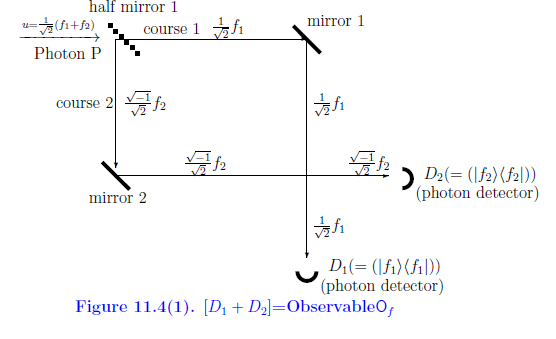
Now we will explain, by the Schrödinger picture, Figure 11.4(1) as follows.
The photon P with the state $u=\frac{1}{\sqrt{2}}( f_1+f_2 )$ ( precisely, $\rho= |u \rangle \langle u |$ ) rushed into the half-mirror 1,
| $(B_1):$ | the $f_1$ part in $u=\frac{1}{\sqrt{2}}( f_1+f_2 )$ passes through the half-mirror 1, and goes along the course 1. And it is reflected in the mirror 1, and goes to the photon detector $D_1$. |
| $(B_2):$ | the $f_2$ part in $u=\frac{1}{\sqrt{2}}( f_1+f_2 )$ rebounds on the half-mirror 1 (and strictly saying, the $f_2$ changes to ${\sqrt{-1}}f_2$, we are not concerned with it ), and goes along the course 2. And it is reflected in the mirror 2, and goes to the photon detector $D_2$. |
This is, by the Heisenberg picture, represented by the following measurement:
\begin{align} {\mathsf M}_{B({\mathbb C}^2)} (\Phi {\mathsf O}_f, S_{[\rho]} ) \tag{11.27} \end{align} Then, we see:| $(C):$ | the probability that $\left[\begin{array}{l} \mbox{ a measured value }1 \\ \mbox{ a measured value }2 \end{array}\right]$ is obtained by $ {\mathsf M}_{B({\mathbb C}^2)} (\Phi {\mathsf O}_f, S_{[\rho]} ) $ is given by \begin{align} \left[\begin{array}{l} \langle Uu, F(\{1\})Uu \rangle \\ \langle Uu, F(\{2\}) Uu \rangle \end{array}\right] = \left[\begin{array}{l} | \langle Uu, f_1 \rangle|^2 \\ | \langle Uu, f_2 \rangle|^2 \end{array}\right] = \left[\begin{array}{l} \frac{1}{2} \\ \frac{1}{2} \end{array}\right] \tag{11.28} \end{align} |
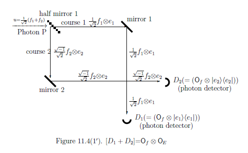
By the analogy of Section 11.2 ( The projection postulate ), Figure 11.4(1) is also described as follows. That is, putting $e_1= \begin{bmatrix} 1 \\ 0 \end{bmatrix} $ and $e_2= \begin{bmatrix} 0 \\ 1 \end{bmatrix} $ $( \in {\mathbb C}^2 )$, we have the observable ${\mathsf O}_E=(\{1,2\},2^{\{1,2\}}, E)$ in $B({\mathbb C}^2)$ such that $E( \{1 \})=|e_1 \rangle \langle e_1$ and $E( \{1 \})=|e_1 \rangle \langle e_1$. Hence,
11.6.4: Mach-Zehnder interferometer (Interference)
Next, consider the following figure:
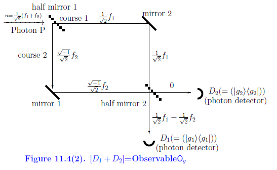
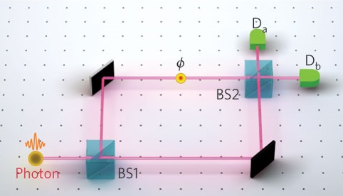
Now we will explain, by the Schrödinger picture, {Figure 11.4(2)} as follows. The photon P with the state $u=\frac{1}{\sqrt{2}}( f_1+f_2 )$ ( precisely, $\rho= |u \rangle \langle u |$ ) rushed into the half-mirror 1,
| $(D1):$ | the $f_1$ part in $u=\frac{1}{\sqrt{2}}( f_1+f_2 )$ passes through the half-mirror 1, and goes along the course 1. And it is reflected in the mirror 1, and passes through the half-mirror 2, and goes to the photon detector $D_1$. |
| $(D2):$ | the $f_2$ part in $u=\frac{1}{\sqrt{2}}( f_1+f_2 )$ rebounds on the half-mirror 1 (and strictly saying, the $f_2$ changes to ${\sqrt{-1}}f_2$, we are not concerned with it ), and goes along the course 2. And it is reflected in the mirror 2, and further reflected in the half-mirror 2, and goes to the photon detector $D_2$. |
This is, by the Heisenberg picture, represented by the following measurement: $ {\mathsf M}_{B({\mathbb C}^2)} (\Phi^2 {\mathsf O}_g, S_{[\rho]} ) $ Then, we see:
| $(E):$ | the probability that $\left[\begin{array}{l} \mbox{ a measured value }1 \\ \mbox{ a measured value }2 \end{array}\right]$ is obtained by $ {\mathsf M}_{B({\mathbb C}^2)} (\Phi^2 {\mathsf O}_g, S_{[\rho]} ) $ is given by \begin{align} \left[\begin{array}{l} \langle u, \Phi^2 G(\{1\})u \rangle \\ \langle u, \Phi^2 G(\{2\}) u \rangle \end{array}\right] =& \left[\begin{array}{ll} | \langle u, UUg_1\rangle |^2 \\ | \langle u, UU g_2 \rangle|^2 \end{array}\right] = \left[\begin{array}{l} 1 \\ 0 \end{array}\right] \tag{11.29} \end{align} |
11.6.5: Another case
Consider the following Figure 11.4(3).
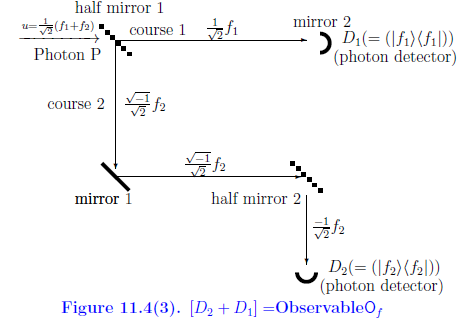
Now we will explain, by the Schrödinger picture, Figure 11.4(3) as follows.
The photon P with the state $u=\frac{1}{\sqrt{2}}( f_1+f_2 )$ ( precisely, $\rho= |u \rangle \langle u |$ ) rushed into the half-mirror 1,
| $(F_1):$ | the $f_1$ part in $u=\frac{1}{\sqrt{2}}( f_1+f_2 )$ passes through the half-mirror 1, and goes along the course 1. And it reaches to the photon detector $D_1$. |
| $(F_2):$ | the $f_2$ part in $u=\frac{1}{\sqrt{2}}( f_1+f_2 )$ rebounds on the half-mirror 1 (and strictly saying, the $f_2$ changes to ${\sqrt{-1}}f_2$, we are not concerned with it ), and goes along the course 2. And it is again reflected in the mirror 1, and further reflected in the half-mirror 2, and goes to the photon detector $D_2$. |
This is, by the Heisenberg picture, represented by the following measurement:
\begin{align} {\mathsf M}_{B({\mathbb C}^2)} (\Phi^2 {\mathsf O}_f, S_{[\rho]} ) \tag{11.30} \end{align}Therefore,we see the following:
| $(F_3):$ |
The probability that
$\left[\begin{array}{l} \mbox{measured value }1 \\ \mbox{measured value }2 \end{array}\right]$
is obtained by
the measurement
$
{\mathsf M}_{B({\mathbb C}^2)} (\Phi^2 {\mathsf O}_f, S_{[\rho]} )
$
is given by
\begin{align}
\left[\begin{array}{l}
\mbox{Tr}(\rho \cdot \Phi^2 F(\{1\}) )
\\
\mbox{Tr}(\rho \cdot \Phi^2 F(\{2\}) )
\end{array}\right]
=
\left[\begin{array}{l}
\langle UUu, F(\{1\})UUu \rangle
\\
\langle UUu, F(\{2\}) UUu \rangle
\end{array}\right]
=
\left[\begin{array}{l}
| \langle UUu, f_1 \rangle|^2
\\
| \langle UUu, f_2 \rangle|^2
\end{array}\right]
=
\left[\begin{array}{l}
\frac{1}{2}
\\
\frac{1}{2}
\end{array}\right]
\end{align}
Therefore,if the photon detector $D_1$ does not react, it is expected that the photon detector $D_2$ reacts. |
The above argument is just Wheeler's delayed choice experiment. It should be noted that the difference among Examples in $\S$11.6.3 (Figure 11.4(1))-- $\S$11.6 (Figure 11.4(3)) is that of the observables (= measuring instrument ). That is,
| $\quad$ | $ \left\{\begin{array}{ll} \mbox{ $\S$11.6.3 (Figure 11.4(1)) } \quad & \xrightarrow[\mbox{ Heisenberg picture}]{} \Phi {\mathsf O}_f \\ \mbox{ $\S$11.6.4 (Figure 11.4(2)) } \quad & \xrightarrow[\mbox{ Heisenberg picture}]{} \Phi^2 {\mathsf O}_g \\ \mbox{ $\S$11.6.5 (Figure 11.4(3)) } \quad & \xrightarrow[\mbox{ Heisenberg picture}]{} \Phi^2 {\mathsf O}_f \end{array}\right. $ |
| $(H):$ |
Wheeler's delayed choice experiment
can not be described paradoxically in quantum language.
Thus, it should be recalled Wittgenstein's famous words:
"Whereof one cannot speak, thereof one must be silent" |
However, it should be noted that the non-locality paradox (i.e., "there is some thing faster than light") is not solved even in quantum language.
| $\fbox{Note 11.3}$ |
What we want to assert in this book may be the following:
|
