You choose randomly (by a fair coin toss) one envelope,
and you get $x_1$ dollars
(i.e.,
if you choose Envelope A [resp.
Envelope B], you get $V_1$ dollars [resp.
$V_2$ dollars]
).
And the host gets $\overline{x}_1$ dollars.
Thus, you can infer that
$\overline{x}_1=2x_1$ or $\overline{x}_1=x_1/2$.
Now the host says
"You are offered the options of keeping your ${x}_1$ or switching to my $\overline{x}_1$".
What should you do?
[(P1):Why is it paradoxical?].
You get $\alpha= x_1$. Then,
you reason that, with probability 1/2, $\overline{x}_1$ is equal to either $\alpha/2$ or $2\alpha$ dollars. Thus the expected value (denoted $E_{\mbox{ other}}(\alpha)$ at this moment) of the other envelope is
\begin{align}
E_{\mbox{ other}}
(\alpha)=(1/2)(\alpha/2) + (1/2)(2\alpha)=1.25\alpha
\tag{9.18}
\end{align}
Consider the state space $\Omega$
such that
with Lebesgue measure $\nu$.
Thus, we start from the classical basic structure
Also, putting
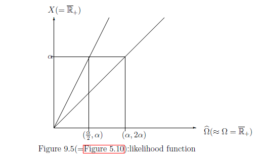
$\widehat{\Omega}=\{ (\omega, 2 \omega ) \;| \; \omega \in \overline{\mathbb R}_+
\}$,
we consider the identification:
Furthermore,
define
$V_1:\Omega (\equiv \overline{\mathbb R}_+) \to X(\equiv \overline{\mathbb R}_+)$
and
$V_2:\Omega (\equiv \overline{\mathbb R}_+) \to X(\equiv \overline{\mathbb R}_+)$
such that
And define the observable
${\mathsf O}=(X(=\overline{\mathbb R}_+), {\mathcal F}(={\mathcal B}_{\overline{\mathbb R}_+}:\mbox{ the Borel field}), F )$
in
$L^\infty (\Omega, \nu )$
such that
The host presents you with a choice between two envelopes
(i.e.,
Envelope A
and
Envelope B). You know one envelope contains twice as much money as the other, but you do not know which contains more. That is, Envelope A [resp.
Envelope B] contains
$V_1$ dollars [resp.
$V_2$ dollars].
You know that
Define the exchanging map $\overline{x}:
\{V_1, V_2 \} \to
\{V_1, V_2\}
$
by
\begin{align}
\overline{x} =
\left\{\begin{array}{ll}
V_2,\;\; (\mbox{ if } x=V_1),
\\
V_1 \;\; (\mbox{ if } x=V_2)
\end{array}\right.
\end{align}
$(a):$
$\qquad
\frac{V_1}{V_2}=1/2$
or,
$\frac{V_1}{V_2}=2$

 This is greater than the $\alpha$ in your current envelope $A$. Therefore,
you should switch to B. But this seems clearly wrong, as your information about A and B is symmetrical.
This is the famous two-envelope paradox
(i.e.,
"The Other Person's Envelope is Always Greener"
).
This is greater than the $\alpha$ in your current envelope $A$. Therefore,
you should switch to B. But this seems clearly wrong, as your information about A and B is symmetrical.
This is the famous two-envelope paradox
(i.e.,
"The Other Person's Envelope is Always Greener"
).
9.5.1:(P1): Bayesian approach to the two envelope problem
Recalling the identification : $\widehat{\Omega} \ni (\omega, 2\omega ) \longleftrightarrow \omega \in \Omega =\overline{\mathbb R}_+$, assume that
\begin{align} \rho_0(D) =\int_D w_0(\omega ) d \omega \quad (\forall D \in {\mathcal B}_{\Omega }={\mathcal B}_{\overline{\mathbb R}_+ }) \end{align}where the probability density function $w_0: \Omega ( \approx \overline{\mathbb R}_+ ) \to \overline{\mathbb R}_+ $ is assumed to be continuous positive function. That is, the mixed state $\rho_0 (\in {\mathcal M}^m(\Omega(=\overline{\mathbb R}_+ ) ) )$ has the probability density function $w_0$.
Axiom${}^{{ (m)}}$ 1 ( in $\S$9.1) says that
| $(A_1):$ | The probability $P(\Xi)$ $(\Xi \in {\mathcal B}_X ={\mathcal B}_{\overline{\mathbb R}_+ })$ that a measured value obtained by the mixed measurement ${\mathsf M}_{L^\infty (\Omega, d \omega )} ({\mathsf O}=(X, {\mathcal F}, F ), S_{[\ast]}(\rho_0))$ belongs to $\Xi (\in {\mathcal B}_X ={\mathcal B}_{\overline{\mathbb R}_+ })$ is given by \begin{align} P (\Xi ) & = \int_\Omega [F(\Xi )](\omega ) \rho_0 (d \omega ) = \int_\Omega [F(\Xi )](\omega ) w_0 (\omega ) d \omega \nonumber \\ & = \int_{\Xi} \frac{w_0(x/2 )}{4} + \frac{w_0(x )}{2} \;\; d x \quad (\forall \Xi \in {\mathcal B_{\overline{\mathbb R}_+ }}) \tag{9.20} \end{align} |
Therefore, the expectation is given by
\begin{align} \int_{\overline{\mathbb R}_+} x P(d x ) = \frac{1}{2} \int_{0}^\infty x \cdot \Big( w_0(x/2 )/2 + w_0(x ) \Big) d x = \frac{3}{2} \int_{\overline{\mathbb R}_+} x w_0(x ) d x \tag{9.21} \end{align}Furthermore, Theorem 9.11 ( Bayes' theorem ) says that
| $(A_2):$ | When a measured value $\alpha$ is obtained by the mixed measurement ${\mathsf M}_{L^\infty (\Omega, d \omega )} ({\mathsf O}=(X, {\mathcal F}, F ),$ $ S_{[\ast]}(\rho_0))$, then the post-state $\rho_{\mbox{ post}} (\in {\mathcal M}^m (\Omega ))$ is given by \begin{align} \rho_{\mbox{ post}}^\alpha = \frac{ \frac{w_0(\alpha/2)}{2} } {\frac{h(\alpha/2)}{2} + w_0(\alpha) } \delta_{(\frac{\alpha}{2}, \alpha)} + \frac{ w_0(\alpha) } {\frac{w_0(\alpha/2)}{2} + w_0(\alpha) } \delta_{({\alpha}{},2 \alpha)} \tag{9.22} \end{align} |
| $(A_3):$ | if $[\ast] = $ $ \left\{\begin{array}{ll} \delta_{(\frac{\alpha}{2}, \alpha)} \\ \delta_{({\alpha}{}, 2 \alpha)} \end{array}\right\} $, then you change $ \left\{\begin{array}{ll} \alpha \longrightarrow \frac{\alpha}{2} \\ \alpha \longrightarrow 2{\alpha} \end{array}\right\} $, and thus you get the switching gain $ \left\{\begin{array}{ll} \frac{\alpha}{2} - \alpha (= - \frac{\alpha}{2} ) \\ 2{\alpha} - \alpha (= {\alpha}) \end{array}\right\} $. |
Therefore, the expectation of the switching gain is calculated as follows:
\begin{align} & \int_{\overline{\mathbb R}_+} \Big( (-\frac{\alpha}{2}) \frac{ \frac{w_0(\alpha/2)}{2} } {\frac{w_0(\alpha/2)}{2} + w_0(\alpha) } + \alpha \frac{ w_0(\alpha) } {\frac{w_0(\alpha/2)}{2} + w_0(\alpha) } \Big) P(d \alpha ) \nonumber \\ = & \int_{\overline{\mathbb R}_+} (-\frac{\alpha}{2})\frac{w_0(\alpha/2 )}{4} + \alpha \cdot \frac{w_0(\alpha )}{2} \;\; d \alpha =0 \tag{9.23} \end{align}Therefore, we see that the swapping is even, i.e., no advantage and no disadvantage.
