9.2: Simple examples in mixed measurement theory
Thus, in what follows I do it
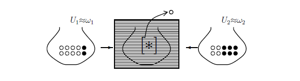
Let us start fron the following review in $\S$5.2:
You do not know which the urn behind the curtain is,
$U_1$ or $U_2$.
Assume that you pick up a white ball from the urn.
The urn is $U_1$ or $U_2$? $\quad$ Which do you think?
Answer:
Consider the state space $\Omega=\{\omega_1, \omega_2\}$
with the discrete topology
and the measure
$\nu$
such that
In the classical basic structure
$
[C_0(\Omega) \subseteq L^\infty (\Omega, \nu ) \subseteq B(L^2 (\Omega, \nu ))]
$,
consider the measurement
${\mathsf M}_{{L^\infty (\Omega) }} ({\mathsf O} {{=}}$
$
( \{ W,$
$ B \},$
$ 2^{\{ W, B \} } ,$
$ F_{WB})
,
S_{ [{}{\ast}]})$,
where
the observable
${\mathsf O}_{WB} = ( \{ W,B \}, 2^{\{ W,B \} } , F_{WB})$
in
$L^\infty (\Omega)$
is defined by
Here, we see:
Then,
Fisher's maximum likelihood method (Theorem 5.6)
says that
Therefore, there is a reason
to infer that
the urn behind the curtain is
$U_1$.
Recall the following wise sayings:
$\quad$
experience is the best teacher,
or
custom makes all things
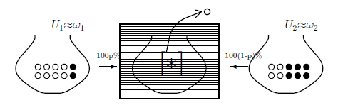
| $(\sharp_1):$ | Assume an unfair coin-tossing
$(T_{p,1-p})$
such that
$( 0 {{\; \leqq \;}}p {{\; \leqq \;}}1 )$:
That is,
$\quad$ $ \left\{\begin{array}{ll} \mbox{the possibility that "head" appears is} \mbox{ $100p \% $} \\ \mbox{the possibility that "tail" appears is} \mbox{ $100(1-p) \% $} \end{array}\right. $ If "head" [resp. "tail"]appears, put an urn $U_1({\approx} \omega_1)$ [resp. $U_2({\approx} \omega_2)$] behind the curtain. Assume that you do not know which urn is behind the curtain, $U_1$ or $U_2$). The unknown urn is denoted by $[*{}](\in \{\omega_1, \omega_2\})$. This situation is represented by $w \in L^1_{+1}(\Omega, \nu )$ (with the counting measure $\nu$), that is, \begin{align} w(\omega ) = \left\{\begin{array}{ll} p \qquad & \mbox{( if $\omega=\omega_1 $ )} \\ 1-p \qquad & \mbox{( if $\omega=\omega_2 $ )} \end{array}\right. \end{align} |
| $(\sharp_2):$ | Consider the "measurement" such that a ball is picked out from the unknown urn. This "measurement" is denoted by ${\mathsf M}_{L^\infty (\Omega,\nu)}({\mathsf O}, {\overline S}_{[*]}(w))$, and called a mixed measurement. |
Then, we have the following problems:
| $(a):$ | Calculate the probability that a white ball is picked from the unknown urm behind the curtain! |
| $(b):$ | when a white ball is picked, calculate the probability that the unknown urm behind the curtain is $U_1$! |
We would like to remark as follows.
| $\bullet$ | in the above problem, the term "subject probability" is not used. |
Answer: Asssume that the state space$\Omega=\{\omega_1, \omega_2\}$ is defined by the discrete metric with the following measure $\nu$: \begin{align} \nu(\{ \omega_1 \})=1, \qquad \nu(\{ \omega_2 \})=1 \tag{9.5} \end{align} Thus, we start from the clasical basic structure: \begin{align} [C_0(\Omega) \subseteq L^\infty (\Omega, \nu ) \subseteq B(L^2 (\Omega, \nu ))] \tag{9.6} \end{align}
in which we consider the mixed measurement ${\mathsf M}_{{L^\infty (\Omega) }} ({\mathsf O} {{=}}$ $ ( \{ W,$ $ B \},$ $ 2^{\{ W, B \} } ,$ $ F) , S_{ [{}{\ast}]}{(w)})$. Here, the observable ${\mathsf O}_{WB} = ( \{ W, B \}, 2^{\{ W, B \} } , F_{WB})$ in $L^\infty (\Omega)$ is defined by
\begin{align} & [F_{WB}(\{ W \})](\omega_1)= 0.8, & \quad & [ F_{WB}(\{ B \})](\omega_1)= 0.2 \nonumber \\ & [F_{WB}(\{ W \})](\omega_2)= 0.4, & \quad & [F_{WB}(\{ B \})] (\omega_2)= 0.6 \tag{9.7} \end{align}Also,the mixed state $w_0 \in L^1_{+1}(\Omega , \nu )$ is defined by
\begin{align} w_0(\omega_1 ) = p, \qquad w_0(\omega_2)=1-p \tag{9.8} \end{align}Then, by Axiom$^{(m)}$1 ( in $\S$9.1), we see
| $(a):$ | the probability that a measured value $x$ $(\in \{ W , B \})$ is obtained by ${\mathsf M}_{{L^\infty (\Omega) }} ({\mathsf O} {{=}}$ $ ( \{ W,$ $ B \},$ $ 2^{\{ W, B \} } ,$ $ F) , S_{ [{}{\ast}]}{(w)})$ is given by |
The question (b) will be answered in Answer9.13.
| $\fbox{Note 9.1}$ |
The following question is natural.
That is,
|
Example 9.6 [Mixed spin measurement ${\mathsf M}_{B({\mathbb C}^2)} ({\mathsf O}=(X= \{ \uparrow, \downarrow \} ,{2}^X, F^z ) , {\overline S}_{[\ast]} (w) )$]
Consider the quantum basic structure: \begin{align} [{\mathcal C}({\mathbb C}^2) ( = B({\mathbb C}^2) ) \subseteq B({\mathbb C}^2) \subseteq B({\mathbb C}^2)] \end{align}And consider a particle $P_1$ with spin state $\rho_1=|a \rangle \langle a|$ $\in$ ${\frak S}^p(B({\mathbb C}^2))$, where
\begin{align} a= \left[\begin{array}{l} \alpha_1 \\ \alpha_2 \end{array}\right] \in {\mathbb C}^2 \quad (\mbox{ }\|a \|= (|\alpha_1|^2+ |\alpha_2|^2)^{1/2}=1) \end{align}And consider another particle $P_2$ with spin state $\rho_2=|b \rangle \langle b|$ $\in$ ${\frak S}^p(B({\mathbb C}^2))$, where
\begin{align} b= \left[\begin{array}{l} \beta_1 \\ \beta_2 \end{array}\right] \in {\mathbb C}^2 \quad (\mbox{ }\|b \|= (|\beta_1|^2+ |\beta_2|^2)^{1/2}=1) \end{align} Here, assume that| $\bullet$ | the "probability" that the "particle" $P$ is $ \left\{\begin{array}{ll} \mbox{ a particle }P_1 \\ \mbox{ a particle } P_2 \end{array}\right\} $ is given by $ \left\{\begin{array}{ll} p \\ 1-p \end{array}\right\} $ |
Here, the unknown state $[\ast]$ of Particle $P$ is represented by the mixed state$w$ $( \in$ ${\frak S}^m ({\mathcal Tr}({\mathbb C}^2)))$ such that
\begin{align} w=p \rho_1 + (1-p) \rho_2 =p |a \rangle \langle a | + (1-p) |b \rangle \langle b| \end{align}Therefore, we have the mixed measurement ${\mathsf M_{B({\mathbb C}^2)}}({\mathsf O}_z =(X,2^X, F^z ), {\overline S}_{[\ast]}(w))$ of the $z$-axis spin observable ${\mathsf O}_z =(X,{\mathcal F}, F^z )$, where
\begin{align} F^z( \{ \uparrow \}) = \left[\begin{array}{ll} 1 & 0 \\ 0 & 0 \end{array}\right] , \quad F^z( \{ \downarrow \}) = \left[\begin{array}{ll} 0 & 0 \\ 0 & 1 \end{array}\right] \end{align} And we say that| $(a):$ | the probability that a measured value $ \left\{\begin{array}{ll} \uparrow \\ \downarrow \end{array}\right\} $ is obtained by the mixed measurement ${\mathsf M_{B({\mathbb C}^2)}}({\mathsf O}_z =(X,2^X, F^z ), {\overline S}_{[\ast]}(w))$ is given by \begin{align} \left\{\begin{array}{ll} {}_{{\mathcal Tr}({\mathbb C}^2)} \Big(w, F^z( \{ \uparrow \}) \Big) {}_{B({\mathbb C}^2)} = p|\alpha_1|^2 +(1-p) |\beta_1|^2 \\ \\ {}_{{\mathcal Tr}({\mathbb C}^2)} \Big(w, F^z( \{ \downarrow \}) \Big) {}_{B({\mathbb C}^2)} = p |\alpha_2|^2 + (1-p)|\beta_2|^2 \end{array}\right\} \end{align} |
As seen in the above, we say that
| $(a):$ | Pure measurement theory is fundamental. Adding the concept of "mixed state", we can construct mixed measurement theory as follows. \begin{align} \underset{\mbox{ ${\mathsf M}_{L^\infty (\Omega)} ({\mathsf O} , {\overline S}_{[\ast ]}{(w)}) $}}{\mbox{$\fbox{ mixed measurement theory }$}} := { { \underset{\mbox{ ${\mathsf M}_{L^\infty (\Omega)} ({\mathsf O} , S_{[\ast ]}) $}}{\mbox{ $\fbox{ pure measurement theory }$}}} } + { { \underset{\mbox{ $w$}} {\mbox{$\fbox{ mixed state}$}} } } \end{align} |
