6.2: The reverse relation between confidence interval method and statistical hypothesis testing
Consider an observable ${\mathsf O} = (X, {\cal F} , F){}$ in ${L^\infty (\Omega)}$. Let $\Theta$ be a locally compact space (called the second state space) which has the
semi-metric
$d^x_{\Theta}$ $(\forall x \in X)$ such that,
Furthermore, consider two maps $E:X \to \Theta$ and $\pi: \Omega \to \Theta$. Here, $E:X \to \Theta$ and $\pi: \Omega \to \Theta$ is respectively called an estimator
and a system quantity
Remark 6.4 [(B$_1$):The meaning of confidence interval]. Consider the parallel measurement $\bigotimes_{j=1}^J {\mathsf M}_{L^\infty (\Omega)} \big({\mathsf O}:= (X, {\cal F} , F) ,$ $ S_{[\omega_0 {}] } \big)$, and assume that a measured value $x=(x_1,x_2, \ldots , x_J)( \in X^J)$ is obtained by the parallel measurement. Recall the formula (6.12). Then, it surely holds that
where $\mbox{Num} [A]$ is the number of the elements of the set $A$. Hence Theorem 6.3 can be tested by numerical analysis (with random number). Similarly, Theorem 6.5 ( mentioned later ) can be tested.
6.2.2 Statistical hypothesis testing
Next, we will explain the statistical hypothesis testing, which is characterized as the reverse of the confident interval method.
Let $0 < \alpha \ll 1$. Consider an observable ${\mathsf O} = (X, {\cal F} , F){}$ in ${L^\infty (\Omega)}$, and the second state space $\Theta$ (i.e., locally compact space with a semi-metric $d_\Theta^x (x \in X)$ ). And consider the estimator $E:X \to \Theta$ and the system quantity $\pi: \Omega \to \Theta$. Define $\delta_\omega^{1-\alpha}$ by (6.9), and define $\eta_\omega^{\alpha}$ by (6.15) ( and thus, $\delta_\omega^{1-\alpha}= \eta_\omega^{\alpha}$).
$(\sharp):$ for each $x\in X$, the map $d^x_{\Theta}: \Theta^2 \to [0,\infty)$ satisfies
(i):$d^x_\Theta (\theta, \theta )=0$,
(ii):$d^x_\Theta (\theta_1, \theta_2 )$ $=d^x_\Theta (\theta_2, \theta_1 )$,
(ii):$d^x_\Theta (\theta_1, \theta_3 )$ $\le d^x_\Theta (\theta_1, \theta_2 ) + d^x_\Theta (\theta_2, \theta_3 ) $.

\begin{align}
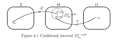
d^x_\Theta (E(x), \pi(\omega_0)) \le {\delta }^{1 -\alpha }_{\omega_0}
\tag{6.10}
\end{align}
And further, put
\begin{align}
D_{x}^{{1 -\alpha, \Theta }}
=
\{
\pi(\omega)
(\in
\Theta)
:
d^x_\Theta (E(x),
\pi(\omega )
)
\le
\delta^{1-\alpha}_{\omega }
\}.
\tag{6.11}
\end{align}
which is called $({1 -\alpha })$-confidence interval.
Here, we see the following equivalence:
\begin{align}
(6.10) \; \Longleftrightarrow \;
\;
D_{x}^{1 -\alpha, \Theta }
\ni
\pi (\omega_0).
\tag{6.12}
\end{align}
$(A):$ the probability, that the measured value $x$ obtained by the measurement ${\mathsf M}_{L^\infty (\Omega)} \big({\mathsf O}:= (X, {\cal F} , F) ,$ $ S_{[\omega_0 {}] } \big)$ satisfies the following condition (6.10), is more than or equal to ${1 -\alpha }$ (e.g., ${1 -\alpha }= 0.95$).
[(B$_2$)] Also, note that
\begin{align}
(6.9)
&
=
\delta_\omega^{1-\alpha}
=
\inf
\{
\delta > 0:
[F(\{ x \in X \;:\;
d^x_\Theta ( E(x) , \pi( \omega ) )
< \delta
\}
)](\omega )
\ge {1-\alpha}
\}
\nonumber
\\
&=
\inf
\{
\eta > 0:
[F(\{ x \in X \;:\;
d^x_\Theta ( E(x) , \pi( \omega ) )
\ge \eta
\}
)](\omega )
\le \alpha
\}
\tag{6.14}
\end{align}

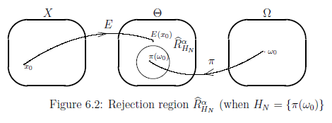
Furthermore, consider a subset $H_N $ of $\Theta$, which is called a "null hypothesis". Put
\begin{align}
&
{\widehat R}_{H_N}^{\alpha, \Theta}
=
\bigcap_{\omega \in \Omega \mbox{ such that }
\pi(\omega) \in {H_N}}
\{
E({x})
(\in
\Theta)
:
d^x_\Theta (E(x),
\pi(\omega )
)
\ge
\eta^\alpha_{\omega }
\}.
\\
&
\tag{6.17}
\end{align}
which is called the $(\alpha)$-rejection region of the null hypothesis ${H_N}$.
Then we say that:
$(C):$ the probability, that the measured value $x$ obtained by the measurement ${\mathsf M}_{L^\infty (\Omega)} \big({\mathsf O}:= (X, {\cal F} , F) ,$ $ S_{[\omega_0 {}] } \big)$ satisfies the following condition (6.16), is less than or equal to $\alpha$ (e.g., $\alpha= 0.05$).
\begin{align}
d^x_\Theta (E(x), \pi(\omega_0)) \ge {\eta }^\alpha_{\omega_0} .
\tag{6.16}
\end{align}
\begin{align}
{\widehat R}_{H_N}^\alpha
\ni
E(x).
\tag{6.18}
\end{align}
$(D):$ the probability, that the measured value $x$ obtained by the measurement ${\mathsf M}_{L^\infty (\Omega)} \big({\mathsf O}:= (X, {\cal F} , F) ,$ $ S_{[\omega_0 {}] } \big)$ $($where $\pi(\omega_0) \in H_N )$ satisfies the following condition (6.18), is less than or equal to $\alpha$ (e.g., $\alpha= 0.05$).
And,
$(E):$ [Confidence interval method]. for each $x \in X$,define $(1- \alpha)$-confidence interval by
\begin{align}
&
D_{x}^{1- \alpha, \Theta }
=
\{
\pi(\omega)
(\in
\Theta)
:
d^x_\Theta (E(x),
\pi(\omega )
)
<
\delta^{1- \alpha}_{\omega }
\}
\tag{6.19}
\end{align}
\begin{align}
&
D_{x}^{1- \alpha, \Omega}
=
\{
\omega
(\in
\Omega)
:
d^x_\Theta (E(x),
\pi(\omega )
)
<
\delta^{1- \alpha}_{\omega }
\}
\tag{6.20}
\end{align}
Here, assume that a measured value $x (\in X)$ is obtained by the measurement ${\mathsf M}_{L^\infty (\Omega)} \big({\mathsf O}:= (X, {\cal F} , F) ,$ $ S_{[\omega_0 {}] } \big)$. Then, we see that
$(E_1):$ the probability that
\begin{align}
D_x^{1-\alpha, \Theta} \ni \pi(\omega_0)
\quad
\mbox{ or,in the same sense }
\quad
D_x^{1-\alpha, \Omega} \ni \omega_0
\end{align}
is more than $1- \alpha$.
$(F):$ [statistical hypothesis testing]. Consider the null hypothesis $H_N ( \subseteq \Theta )$. Assume that the state $\omega_0(\in \Omega )$ satisfies:
\begin{align}
\pi(\omega_0)
\in
H_N
( \subseteq \Theta )
\end{align}
Here, put,
\begin{align}
&
{\widehat R}_{{H_N}}^{\alpha; \Theta}
=
\bigcap_{\omega \in \Omega \mbox{ such that }
\pi(\omega) \in {H_N}}
\{
E({x})
(\in
\Theta)
:
d^x_\Theta (E(x),
\pi(\omega )
)
\ge
\eta^\alpha_{\omega }
\}.
\\
&
\tag{6.21}
\end{align}
\begin{align}
&
{\widehat R}_{{H_N}}^{\alpha; X}
=
E^{-1}(
{\widehat R}_{{H_N}}^{\alpha; \Theta})
=
\bigcap_{\omega \in \Omega \mbox{ such that }
\pi(\omega) \in {H_N}}
\{
x
(\in
X)
:
d^x_\Theta (E(x),
\pi(\omega )
)
\ge
\eta^\alpha_{\omega }
\}.
\\
&
\tag{6.22}
\end{align}
which is called the $(\alpha)$-rejection region of the null hypothesis ${H_N}$.
Assume that a measured value $x (\in X)$ is obtained by the measurement ${\mathsf M}_{L^\infty (\Omega)} \big({\mathsf O}:= (X, {\cal F} , F) ,$ $ S_{[\omega_0 {}] } \big)$. Then, we see that
$(F_1):$ the probability that
\begin{align}
&
"E(x) \in
{\widehat R}_{{H_N}}^{\alpha; \Theta}"
\quad
\mbox{ or,in the same sense, }
\quad
"x
\in
{\widehat R}_{{H_N}}^{\alpha; X}"
\\
&
\tag{6.23}
\end{align}
is less than $\alpha$.
6.2: The reverse relation between confidence interval method and statistical hypothesis testing
This web-site is the html version of "Linguistic Copehagen interpretation of quantum mechanics; Quantum language [Ver. 4]" (by Shiro Ishikawa; [home page] )
PDF download : KSTS/RR-18/002 (Research Report in Dept. Math, Keio Univ. 2018, 464 pages)
Contents:
In what follows, we shall mention the reverse relation (such as "the two sides of a coin") between confidence interval method and statistical hypothesis testing.
We devote ourselves to the classical systems, i.e., the classical basic structure:
\begin{align}
[ C_0(\Omega ) \subseteq L^\infty (\Omega, \nu ) \subseteq B(L^2 (\Omega, \nu ))]
\end{align}
6.2.1: The confidence interval method
Theorem 6.3 [Confidence interval method].
Let a positive number $\alpha$ be $0 < \alpha \ll 1$, for example, $\alpha = 0.05$. For any state $ \omega (\in \Omega)$, define the positive number $\delta^{1-\alpha}_{\omega}$ $(> 0)$ such that:
\begin{align}
\delta^{1-\alpha}_{\omega}
=
\inf
\{
\delta > 0:
[F(\{ x \in X \;:\;
d^x_\Theta ( E(x) , \pi( \omega ) )
< \delta
\}
)](\omega )
\ge {1 -\alpha }
\}
\\
&
\tag{6.9}
\end{align}
Then we say that:
Theorem 6.5 [Statistical hypothesis testing]
Let $\alpha$ be a real number such that $0 < \alpha \ll 1$, for example, $\alpha = 0.05$. For any state $ \omega (\in \Omega)$, define the positive number $\eta^\alpha_{\omega}$ $(> 0)$ such that:
\begin{align}
\eta^\alpha_{\omega}
&
=
\inf
\{
\eta > 0:
[F(\{ x \in X \;:\;
d^x_\Theta ( E(x) , \pi( \omega ) )
\ge \eta
\}
)](\omega )
\le \alpha
\}
\tag{6.15}
\\
&
\mbox{
( by the (6.14), note that $\delta_\omega^{1 - \alpha}=\eta_\omega^\alpha$)
}
\nonumber
\end{align}
Then we say that:
6.2.3: The reverse relation between Confidence interval and statistical hypothesis testing
Corollary6.6[The reverse relation between Confidence intervaland statistical hypothesis testing]
