All examples mentioned in this section are easy for the readers who studied the elementary of statistics. However, it should be noted that these are consequence of Axiom 1 ( measurement: $\S$2.7).
Furthermore,
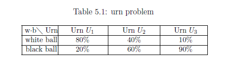
$(i):$ one of three urns is chosen, but you do not know it. Pick up one ball from the unknown urn. And you find that its ball is white. Then, how do you infer the unknown urn, i.e., $U_1$, $U_2$ or $U_3$?
In what follows, we shall answer the above problems (i) and (ii) in terms of measurement theory. Consider the classical basic structure:
\begin{align}
\mbox{
$[C_0(\Omega ) \subseteq L^\infty (\Omega, \nu ) \subseteq B(L^2(\Omega, \nu ))]$}
\end{align}
Put
\begin{align}
\delta_{\omega_j}(\approx \omega_j )
\longleftrightarrow
[
\mbox{the state such that urn $U_j$ is chosen}
]
\quad
(j=1,2,3)
\end{align}
Thus, we have the state space $\Omega$ $($ ${{=}} \{ \omega_1 , \omega_2 , \omega_3 \}$ $)$ with the counting measure $\nu$. Furthermore, define the observable ${\mathsf O} = ( \{ {{w}}, {{b}} \}, 2^{\{ {{w}}, {{b}} \} } , F)$ in $C(\Omega)$ such that
\begin{align}
& F(\{ {{w}} \})(\omega_1)= 0.8, & \;\;\;&
& F(\{ {{w}} \})(\omega_2)= 0.4, & \;\;\;&
& F(\{ {{w}} \})(\omega_3)= 0.1 \\
& F(\{ {{b}} \})(\omega_1)= 0.2, & \;\;\;&
& F(\{ {{b}} \})(\omega_2)= 0.6, & \;\;\;&
& F(\{ {{b}} \})(\omega_3)= 0.9
\end{align}
Answer to (i):
Consider the measurement ${\mathsf M}_{L^\infty (\Omega)} ({\mathsf O}, S_{[{}\ast{}]})$, by which a measured value "w" is obtained. Therefore, we see
\begin{align}
[F({ \{ {{w}} \} })] (\omega_1) =
0.8
=
\max_{ \omega \in \Omega }
[F({ \{ {{w}} \} })] (\omega)
=
\max
\{ 0.8, \; 0.4, \; 0.1 \}
\end{align}
Hence, by Fisher's maximum likelihood method (Theorem5.6) we see that
\begin{align}
[\ast] = \omega_1
\end{align}
Thus, we can infer that the unknown urn is $U_1$.
$(ii):$ And further, you pick up another ball from the unknown urn (in (i)). And you find that its ball is black. That is, after all, you have one white ball and one black ball. Then, how do you infer the unknown urn, i.e., $U_1$, $U_2$ or $U_3$?
Answer to (ii):
Next, consider the simultaneous measurement ${\mathsf M}_{L^\infty (\Omega)} (\times_{k=1}^2 {\mathsf O} $ $ {{=}} $ $ (X^2 ,$ $ 2^{{}X^2} ,$ $ {\widehat F} {{=}} \times_{k=1}^2 F) ,$ $ S_{[{}\ast]})$, by which a measured value $( {{w}}, {{b}})$ is obtained. Here, we see
\begin{align}
[{\widehat F}(\{({{w}},{{b}})\})](\omega)=[F({\{{{w}}\}})](\omega)
\cdot
[F({\{{{b}}\}})](\omega)
\end{align}
thus,
\begin{align}
&[{\widehat F}(\{({{w}},{{b}})\})](\omega_1)=0.16,
\;\;
[{\widehat F}(\{({{w}},{{b}})\})](\omega_2)= 0.24,
\;\;
[{\widehat F}(\{({{w}},{{b}})\})](\omega_3)= 0.09
\end{align}
Hence, by Fisher's maximum likelihood method (Theorem5.6), we see that
\begin{align}
[\ast] = \omega_2
\end{align}
Thus, we can infer that the unknown urn is $U_2$.
Answer(a): Put
\begin{align}
\Xi_i = [ x_i^0 -\frac{1}{N},x_i^0 +\frac{1}{N}]
\qquad(i=1,2,3)
\end{align}
Assume that $N$ is sufficiently large. Fisher's maximum likelihood method (Theorem5.6) says that the unknown state $[{}\ast{}]$ $= \mu_0$ is found in what follows.
\begin{align}
[G_{\sigma}^3({\Xi_1 \times \Xi_2 \times \Xi_3 })] ( {\mu_0} )
=
\max_{\mu \in {\mathbb R}}
[G_{\sigma}^3({\Xi_1 \times \Xi_2 \times \Xi_3 })] ( {\mu} )
\end{align}
Since $N$ is sufficiently large, we see
\begin{align}
&
\frac{1}{({\sqrt{2 \pi } \sigma)^3}}
\exp[{}- \frac{({x^0_1} - {\mu_0} )^2 +({x^0_2} - {\mu_0} )^2 +
({x^0_3} - {\mu_0} )^2 }{2 \sigma^2 }
]
\\
=
&
\max_{\mu \in {\mathbb R}}
\Big[
\frac{1}{({\sqrt{2 \pi } \sigma)^3}}
\exp[{}- \frac{({x^0_1} - {\mu} )^2 +({x^0_2} - {\mu} )^2 +
({x^0_3} - {\mu} )^2 }{2 \sigma^2 }
]
\Big]
\end{align}
That is,
\begin{align}
({x^0_1} - {\mu_0} )^2 +({x^0_2} - {\mu_0} )^2 +
({x^0_3} - {\mu_0} )^2
=
\min_{\mu \in {\mathbb R}}
\big\{
({x^0_1} - {\mu} )^2 +({x^0_2} - {\mu} )^2 +
({x^0_3} - {\mu} )^2
\big\}
\end{align}
Therefore, solving $\frac{d}{d\mu} \{ \cdots \}=0$, we conclude that
\begin{align}
\mu_0
=
\frac{{x^0_1}+{x^0_2}+{x^0_3}}{3}
\end{align}
[Normal observable (ii)]
Next consider the classical basic structure:
$(a):$ Assume that a measured value $(x^0_1, x^0_2 , x^0_3)$ $(\in {\mathbb R}^3)$ is obtained by the measurement ${\mathsf M}_{L^\infty({\mathbb R})} ({\mathsf O}_{G_\sigma}^3,$ $
S_{[{}\ast{}] })$. Then, infer the unknown state $[\ast] (\in {\mathbb R})$.
 \begin{align}
[ C_0(\Omega ) \subseteq L^\infty (\Omega, \nu ) \subseteq B(L^2 (\Omega, \nu ))]\quad
(\mbox{where ,}
\Omega
=
{\mathbb R} \times {\mathbb R}_+
)
\end{align}
and consider the case:
\begin{align}
[ C_0(\Omega ) \subseteq L^\infty (\Omega, \nu ) \subseteq B(L^2 (\Omega, \nu ))]\quad
(\mbox{where ,}
\Omega
=
{\mathbb R} \times {\mathbb R}_+
)
\end{align}
and consider the case:
And we assume that
$\bullet$ we know that the length of the pencil $\mu$ is satisfied that 10cm $\le $ $\mu$ cm $\le $30cm.
That is, assume that the state space $\Omega$ $=$ $[10,30{}] \times {\mathbb R}_+ $ $
\big(
{{=}}
\{ \mu \in {\mathbb R} \; |\; 10 {{\; \leqq \;}}\mu {{\; \leqq \;}}30 \}
\times
\{ \sigma \in {\mathbb R}
\;|\;
\sigma > 0
\}
\big)
$
Define the observable ${\mathsf O}$ ${{=}}$ $({\mathbb R} , {\cal B}_{{\mathbb R}}^{} , G)$ in $L^\infty ([10,30 {}]\times {\mathbb R}_+)$ such that
\begin{align}
[G(\Xi)](\mu, \sigma )
=
[{G_\sigma}({\Xi})] (\mu)
\quad
(\forall \Xi \in {\cal B}_{{\mathbb R}}^{},
\;\;
\forall ({\mu}, \sigma)
\in
\Omega=
[10,30] \times {\mathbb R}_+
)
\end{align}
Therefore, the simultaneous observable ${\mathsf O}^3 $ ${{=}}$ $({\mathbb R}^3 , {\cal B}_{{\mathbb R}^3}^{} ,$ $ G^3)$ in $C ([10,30{}]\times {\mathbb R}_+)$ is defined by
\begin{align}
&
[G^3({\Xi_1 \times \Xi_2 \times \Xi_3 })] ( {\mu},\sigma )
=
[G(\Xi_1)](\mu, \sigma )
\cdot
[G(\Xi_2)](\mu, \sigma )
\cdot
[G(\Xi_3)](\mu, \sigma )
\\
=
&
\frac{1}{({\sqrt{2 \pi } \sigma)^3}}
\int_{\Xi_1 \times \Xi_2 \times \Xi_3}
\exp[{}- \frac{({x_1} - {\mu} )^2 +({x_2} - {\mu} )^2 +
({x_3} - {\mu} )^2 }{2 \sigma^2 }
] d{x_1} d{x_2} d{x_3}
\\
&
\qquad \qquad \qquad
(\forall \Xi_k \in {\cal B}_{{\mathbb R}}^{},k=1,2,3,
\quad
\forall ({\mu},\sigma) \in \Omega=
[10,30{}]\times {\mathbb R}_+)
\end{align}
Thus, we get the simultaneous measurement ${\mathsf M}_{L^\infty([10,30]\times {\mathbb R}_+)} ({\mathsf O}^3, S_{[{}\ast{}] })$. Here, we have the following problem:
$(\sharp):$ the length of the pencil $\mu$ and the roughness $\sigma$ of the ruler are unknown.
Answer (b):
By the same way of (a), Fisher's maximum likelihood method (Theorem5.6) says that the unknown state $[{}\ast{}]$ $= (\mu_0,\sigma_0)$ such that
\begin{align}
&
\frac{1}{({\sqrt{2 \pi } \sigma_0)^3}}
\exp[{}- \frac{({x^0_1} - {\mu_0} )^2 +({x^0_2} - {\mu_0} )^2 +
({x^0_3} - {\mu_0} )^2 }{2 \sigma_0^2 }
]
\nonumber
\\
=
&
\max_{(\mu,\sigma) \in [10, 30] \times {\mathbb R}_+}
\Big\{
\frac{1}{({\sqrt{2 \pi } \sigma)^3}}
\exp[{}- \frac{({x^0_1} - {\mu} )^2 +({x^0_2} - {\mu} )^2 +
({x^0_3} - {\mu} )^2 }{2 \sigma^2 }
]
\Big\}
\tag{5.12}
\end{align}
Thus, solving $\frac{\partial }{\partial \mu}\{\cdots \}=0$, $\frac{\partial }{\partial \sigma}\{\cdots \}=0$ we see
\begin{align}
&
\mu_0
=
\left\{\begin{array}{ll}
10
\quad
\qquad
&
(\mbox{when }
\mbox{}
(x^0_1+x^0_2+x^0_3)/3< 10\; )
\\
\\
({x^0_1}+{x^0_2}+{x^0_3})/3
\quad
\qquad&
(\mbox{when }
\mbox{}
10 {{\; \leqq \;}}
(x^0_1+x^0_2+x^0_3)/3{{\; \leqq \;}}30 \; \mbox)
\\
\\
30
\quad&
(\mbox{when }
30
<
(x^0_1+x^0_2+x^0_3)/3 \;)
\end{array}\right.
\tag{5.13}
\\
&
\sigma_0
=
\sqrt{
\{
(x^0_1-{\widetilde \mu})^2
+
(x^0_2-{\widetilde \mu})^2
+
(x^0_3-{\widetilde \mu})^2
\}/3
}
\nonumber
\end{align}
where
\begin{equation*}
{\widetilde \mu}=({x^0_1}+{x^0_2}+{x^0_3} )/3
\end{equation*}
$(b):$ When a measured value $(x^0_1, x^0_2 , x^0_3)$ $(\in {\mathbb R}^3)$ is obtained by the measurement ${\mathsf M}_{L^\infty([10,30]\times {\mathbb R}_+)}$ $ ({\mathsf O}^3,$ $ S_{[{}\ast{}] })$, infer the unknown state $[\ast] ( = (\mu_0,\sigma_0) \in [10,30]\times {\mathbb R}_+)$, i.e., the length $\mu_0$ of the pencil and the roughness $\sigma_0$ of the ruler.
5.3: Examples: Fisher's maximum likelihood method
This web-site is the html version of "Linguistic Copehagen interpretation of quantum mechanics; Quantum language [Ver. 4]" (by Shiro Ishikawa; [home page] )
PDF download : KSTS/RR-18/002 (Research Report in Dept. Math, Keio Univ. 2018, 464 pages)
Example 5.8 [Urn problem] Each urn $U_1$, $U_2$, $U_3$ contains many white balls and black ball such as:
Here,
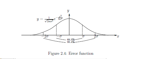
Example 5.9 [Normal observable(i): $\Omega={\mathbb R}$] As mentioned before, we again discuss the normal observable in what follows. Consider the classical basic structure:
\begin{align}
\mbox{
$[ C_0(\Omega ) \subseteq L^\infty (\Omega, \nu ) \subseteq B(L^2 (\Omega, \nu ))]\qquad$
(where,
$\Omega={\mathbb R} )$
}
\end{align}
Fix $\sigma > 0$, and consider the normal observable ${\mathsf O}_{G_\sigma} $ ${{=}}$ $({\mathbb R} , {\cal B}_{{\mathbb R}}^{} , {G_\sigma})$ in $L^\infty ({\mathbb R})$ (where $\Omega={\mathbb R}$) such that
\begin{align}
&[{G_\sigma}(\Xi)] ( {\mu} ) =
\frac{1}{{\sqrt{2 \pi } \sigma}}
\int_{\Xi} \exp[{}- \frac{1}{2 \sigma^2 } ({x} - {\mu} )^2
] d{x}
\\
&
\qquad
(\forall \Xi \in {\cal B}_{{\mathbb R}}^{},
\quad
\forall {\mu} \in \Omega= {\mathbb R})
\end{align}
Thus, the simultaneous observable $\times_{k=1}^3 {\mathsf O}_{G_\sigma}$ (in short, ${\mathsf O}_{G_\sigma}^3 $) ${{=}}$ $({\mathbb R}^3 , {\cal B}_{{\mathbb R}^3}^{} ,$ $ G_{\sigma}^3)$ in $L^\infty ({\mathbb R})$ is defined by
\begin{align}
&
[G_{\sigma}^3({\Xi_1 \times \Xi_2 \times \Xi_3 })] ( {\mu} )
=
[{G_\sigma}({\Xi_1})] (\mu) \cdot
[{G_\sigma}({\Xi_2})] (\mu) \cdot
[{G_\sigma}({\Xi_3})](\mu)
\\
=
&
\frac{1}{({\sqrt{2 \pi } \sigma)^3}}
\iiint_{\Xi_1 \times \Xi_2 \times \Xi_3}
\exp[{}- \frac{({x_1} - {\mu} )^2 +({x_2} - {\mu} )^2 +
({x_3} - {\mu} )^2 }{2 \sigma^2 }
] \\
&\hspace{5cm} \times d{x_1} d{x_2} d{x_3}
\\
&
\qquad \qquad \qquad \qquad
(\forall \Xi_k \in {\cal B}_{{\mathbb R}}^{},k=1,2,3,
\quad
\forall {\mu} \in \Omega= {\mathbb R})
\end{align}
Thus, we get the measurement ${\mathsf M}_{L^\infty({\mathbb R})} ({\mathsf O}_{G_\sigma}^3, S_{[{}\ast{}] })$
Now we consider the following problem:
Example 5.10 [Fisher's maximum likelihood method for the simultaneous normal measurement]
Consider the simultaneous normal observable ${\mathsf O}_G^n = ({\mathbb R}^n, {\mathcal B}_{\mathbb R}^n, {{{G}}^n} )$ in $L^\infty ({\mathbb R} \times {\mathbb R}_+)$ (such as defined in formula (5.3). This is essentially the same as the simultaneous observable ${\mathsf O}^n$ $=$ $({\mathbb R}^n, {\mathcal B}_{{\mathbb R}^n}, \times_{k=1}^n {G_\sigma})$ in $L^\infty ({\mathbb R} \times {\mathbb R}_+)$. That is,
\begin{align}
&
[(\times_{k=1}^n {G_\sigma})(\Xi_1 \times \Xi_2 \times
\cdots \times \Xi_n )](\omega)
=
\times_{k=1}^n [G_{\sigma}(\Xi_k) ]( {\omega} )
\nonumber
\\
=
&
\times_{k=1}^n
\frac{1}{{\sqrt{2 \pi } \sigma}}
\int_{\Xi_k} \exp
\left[
{}- \frac{1}{2 \sigma^2 } ({x_k} - {\mu} )^2
\right] d{x_k}
\nonumber
\\
&
\quad
(\forall \Xi_k \in {\cal B}_{{X}}^{}( ={\cal B}_{{\mathbb R}}^),
\;
\forall {\omega}=(\mu, \sigma ) \in \Omega (={\mathbb R}\times {\mathbb R}_+ ))
\nonumber
\end{align}
Assume that a measured value $x=(x_1, x_2, \ldots, x_n ) (\in {\mathbb R}^n )$ is obtained by the measurement ${\mathsf M}_{L^\infty ({\mathbb R} \times {\mathbb R}_+ )} ({\mathsf O}^n = ({\mathbb R}^n, {\mathcal B}_{\mathbb R}^n, {{{G}}_\sigma^n} )$,$S_{[\ast]})$. The likelihood function $L_x(\mu, \sigma)(=L(x, (\mu,\sigma)) $ is equal to
\begin{align}
L_x(\mu, \sigma)
&
=
\frac{1}{({{\sqrt{2 \pi }\sigma{}}})^n}
\exp[{}- \frac{\sum_{k=1}^n ({}{x_k} - {}{\mu} )^2
}
{2 \sigma^2} {}]
\nonumber
\end{align}
in the sense of (5.9),
\begin{align}
L_x(\mu, \sigma)
&
=
\frac{
\frac{1}{({{\sqrt{2 \pi }\sigma{}}})^n}
\exp[{}- \frac{\sum_{k=1}^n ({}{x_k} - {}{\mu} )^2
}
{2 \sigma^2} {}] }
{
\frac{1}{({{\sqrt{2 \pi }\overline{\sigma}(x){}}})^n}
\exp[{}- \frac{\sum_{k=1}^n ({}{x_k} - {}{\overline{\mu}(x)} )^2
}
{2 \overline{\sigma}(x)^2} {}]
}
\\
&
(\forall x = (x_1, x_2, \ldots , x_n ) \in {\mathbb R}^n,
\quad
\forall {}{\omega}=(\mu, \sigma ) \in \Omega = {\mathbb R}\times {\mathbb R}_+).
\end{align}
Therefore,we get the following likelihood equation:
\begin{align}
\frac{\partial L_x(\mu, \sigma)}{\partial \mu}=0,
\quad
\frac{\partial L_x(\mu, \sigma)}{\partial \sigma}=0
\tag{5.15}
\end{align}
which is easily solved. That is, Fisher's maximum likelihood method (Theorem5.6) says that the unknown state $[\ast]=(\mu, \sigma)$ $(\in {\mathbb R} \times {\mathbb R}_+)$ is inferred as follows.
\begin{align}
&
\mu=\overline{\mu}(x) =\frac{x_1 + x_2+ \ldots + x_n }{n},
\quad
\tag{5.16}
\\
&
\sigma=
\overline{\sigma}(x)
=
\sqrt{\frac{\sum_{k=1}^n (x_k - \overline{\mu}(x))^2}{n}}
\tag{5.17}
\end{align}
