In the previous section, we studied the above $(\sharp_1)$, that is, we discussed the following classification:
In this section, we shall study the above $(\sharp_2)$, i.e.,
2.4.1 Dualism (John Locke)
Our present purpose is to learnAxiom 1 ( measurement ) by rote
The "learning by rote" urges us to understand the mathematical definitions
of
$(\sharp_1):$ Basic structure$[ {\mathcal A} \subseteq \overline{\mathcal A}]_{B(H)}$, state space ${\frak S}^p({\cal A}^*)$
$(\sharp_2):$ observable ${\mathsf O}{{=}} (X, {\cal F} , F{})$, etc.
(B): $\underset{\mbox{ state space }[{\frak S}^p({\cal A}^*),{\frak S}^m({\cal A}^*),\overline{\frak S}^p(\overline{\cal A}_*)]}{\mbox{General basic structure}[ {\mathcal A} \subseteq \overline{\mathcal A}]_{B(H)}}$
$\quad \qquad
\Longrightarrow
\left\{\begin{array}{ll}
\underset{\mbox{ state space }[{\frak S}^p({\mathcal Tr}(H)),{\frak S}^m({\mathcal Tr}(H))= \overline{\frak S}^m({\mathcal Tr}(H))]}{\mbox{Quantum basic structure}[ {\mathcal C}(H) \subseteq B(H)]_{B(H)}}
\\
\\
\\
\underset{\mbox{ state space }[\Omega, {\mathcal M}_{+1}(\Omega),L^\infty(\Omega, \nu )
]}{\mbox{Classical basic structure}[ C_0(\Omega) \subseteq L^\infty(\Omega, \nu )]_{B(L^2(\Omega, \nu ))}}
\end{array}\right.
$
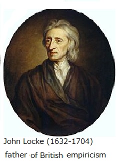
Recall the famous words: "the primary quality"and "the secondary quality" due to John Locke,an English philosopher and physician regarded as one of the most influential of Enlightenment thinkers and known as the "Father of British empiricism". We think the following correspondence:
\begin{align}
\left\{\begin{array}{ll}
\mbox{[state]} & \longleftrightarrow \mbox{[the primary quality]}
\\
\mbox{[observable]} & \longleftrightarrow \mbox{[the secondary quality]}
\end{array}\right.
\tag{2.47}
\end{align}
And thus, we think
Also, the following table promotes the better understanding of quantum language as well as the other world-views(i.e., the conventional philosophies).
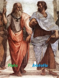
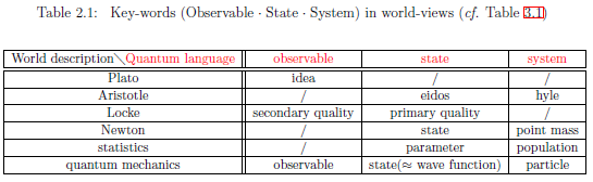
Although I am not familiar with "ontology", I want to consider that "key-word" exists in each world-view
| $\fbox{Note 2.2}$ |
It may be understandable to consider
\begin{align}
\mbox{
"observable" ="the partition of word"="the secondary quality"
}
\end{align}
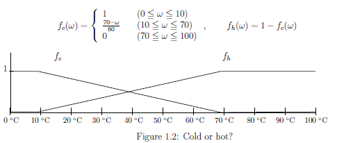
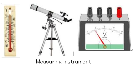
For example, Chapter 1 (Figure 1.2) says that $\big( f_{{c}}, f_{{h}} \big)$ is the partition between "cold" and "hot". Also, "measuring instrument" is the instrument that choose a word among words. In this sense, we consider that "observable"= "measuring instrument". Also, The reason that John Locke's sayings "primary quality (e.g., length, weight, etc.)" and "secondary quality (e.g., sweet, dark, cold, etc.)" is that these words form the basis of dualism. |

2.4.2 Dualism (in philosophy) and duality (in mathematics)
The following question may be significant:| (C1): | Why did philosophers continue persisting in dualism? |
As the typical answer, we may consider that
| (C2): | "I" is the special existence, and thus, we would like to draw a line between "I" and "matter". |
But, we think that this is only quibbling. We want to connect the question (C$_1$) with the following mathematical question:
| (C3): | Why do mathematicians investigate "dual space"? |
Of course, the question "why?" is non-sense in mathematics. If we have to answer this, we have no answer except the following (D):
| (D): | If we consider the dual space ${\mathcal A}^*$, calculation progresses deeply. |
Thus, we want to consider the relation between the dualism and the dual space such as \begin{align} \left\{\begin{array}{ll} \mbox{[the primary quality]} & \longleftrightarrow \mbox{the state in the dual space ${\mathcal A}^*$} \\ \mbox{[the secondary quality]} & \longleftrightarrow \mbox{the observable in $C^*$ algebra ${\mathcal A}$ (or, $W^*$-algebra $\overline{\mathcal A}$)} \end{array}\right. \end{align} Hence, we consider that the answer to the (C$_1$) is also
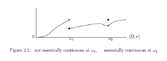
2.4.3 Essentially continuous
In $\S$2.1..2, we introduced the following diagram:| (F1): | if $\rho_n ( \in {\overline{\frak S}^m(\overline{\mathcal A}_*)})$ weakly converges to $\rho_0 (\in {\frak S}^m ({}{\cal A}^*{}))$. That is, $$ \lim_{n \to \infty } {}_{\overline{\mathcal A}_\ast} \Big( \rho_n, G \Big){}_{{\mathcal A}} = {}_{{\mathcal A}^\ast} \Big( \rho_0, G \Big){}_{{\mathcal A}} (\forall G \in {\cal A} (\subseteq \overline{\cal A} ) ), $$ then it holds that $$ \lim_{n \to \infty } {}_{\overline{\mathcal A}_\ast} \Big( \rho_n, F \Big){}_{\overline{\mathcal A}} =\alpha $$ |
Of course, for any $\rho_0 (\in {\frak S}^m ({}{\cal A}^*{}))$, $F (\in {\mathcal A})$ is essentially continuous at $\rho_0$. This "essentially continuous" is chiefly used in th case that $\rho_0 (\in {\frak S}^p ({}{\cal A}^*{}))$.
Remark 2.1 [Essentially continuous in quantum system and classical system] Consider the quantum basic structure $[{\mathcal C}(H) \subseteq B(H)]_{B(H)}$. Then, we see \begin{align*} ({\mathcal C}(H))^*= {\mathcal {\mathcal Tr}(H)} = B(H)_* \end{align*}
Thus, we haven $\rho \in {\frak S}^p({\mathcal C}(H)^*) \subseteq {\mathcal Tr}(H)$, $F \in \overline{{\mathcal C}(H)}=B(H)$, which implies that
\begin{align} \rho(G)= {}_{{\mathcal C}(H)^*} \Big( \rho, F )\Big){}_{B(H)} = {}_{{\mathcal Tr}(H)} \Big( \rho, F )\Big){}_{B(H)} \tag{2.51} \end{align} Thus, we see that "essentially continuous" $\Leftrightarrow$ "continuous" in quantum case.[II]: Next, consider the classical basic structure $[C_0(\Omega ) \subseteq L^\infty (\Omega, \nu ) \subseteq B(L^2 (\Omega, \nu ))]$. A function $F$ $( \in L^\infty ( \Omega, \nu ))$ is essentially continuous at $\omega_0$ $( \in \Omega = {\frak S}^p(C_0(\Omega )^*) )$, if and only if it holds that
| (F2): | if $\rho_n (\in L_{+1}^1(\Omega, \nu )$ satisfies that \begin{align*} \lim_{n \to \infty } \int_\Omega G(\omega ) \rho_n(\omega) \nu (d \omega ) =G(\omega_0) \qquad (\forall G \in C_0(\Omega ) ) \end{align*} then there uniquely exists a complex number $\alpha$ such that \begin{align} \lim_{n \to \infty } \int_\Omega F(\omega) \rho_n (\omega) \nu (d \omega ) = \alpha \tag{2.52} \end{align} |
2.4.4 The definition of "observable (=measuring instrument)"
Let $X$ be a set ( or locally compact space). The ${\cal F}\Big( \subseteq 2^X = {\mathcal P}(X)=\{ A \;|\; A \subseteq X \}, \mbox{the power set of $X$}\Big)$ (or, the pair $(X, {\mathcal F})$) is called a ring ( of sets), if it satisfies that
\begin{align*} & ({\rm a}): \emptyset (\mbox{="empty set"})\in {\cal F}, \quad \\ & ({\rm b}): \Xi_i \in {\cal F} \quad (i=1,2,\ldots) \Longrightarrow { \bigcup\limits_{i=1}^n } \;\; \Xi_i \in {\cal F} ,\quad { \bigcap\limits_{i=1}^n } \;\; \Xi_i \in {\cal F} \\ & ({\rm c}): \Xi_1 , \Xi_2 \in {\cal F} \Longrightarrow \Xi_1 \setminus \Xi_2 \in {\cal F} \quad (\mbox{ where, } \Xi_1 \setminus \Xi_2= \{ x \;| \; x \in \Xi_1 , x \notin \Xi_2 \}) \end{align*}Also, if $X \in {\mathcal F}$ holds, the ring ${\mathcal F}$(or, the pair $(X, {\mathcal F})$) is called a field (of sets) And further,
| (d): | if the formula (b) holds in the case that $n=\infty$, a field ${\mathcal F}$ is said to be $\sigma$-field. And the pair $( X, {\mathcal F} )$ is called a measurable space. |
| $(i)$: | $(X, {\mathcal R})$ is a ring of sets. | ||||||
| $(ii)$: | a map $F: {\cal R} \to {\mathcal A}$ satisfies that
|
(G$_2$):$W^*$- observable A triplet ${\mathsf{O}} {=} (X, {\cal F}, F)$ is called a $W^*$-observable (or, $W^*$-measuring instrument ) in $\overline{\mathcal A}$, if it satisfies as follows.
| $(i)$: | $(X, {\mathcal F})$ is a $\sigma$-field. | ||||||
| $(ii)$: | a map $F: {\cal F} \to \overline{\mathcal A}$
satisfies that
|
| $(\sharp_1)$: | ${\mathcal F}$ is the smallest $\sigma$-field that contains ${\mathcal F}_\rho$. |
| $(\sharp_2)$: | \begin{align} {}_{\stackrel{{}}{{\mathcal A}^* }}\Big(\rho, F(\Xi) \Big){}_{\stackrel{{}}{\overline{\mathcal A} }} = P_\rho (\Xi ) \qquad (\forall \Xi \in {\mathcal F}_\rho ) \end{align} |
Concerning the $C^*$-observable, the sample probability space clearly exists. On the other hand, concerning the $W^*$-observable, we have to say something as follows. As mentioned in Remark 2.15, in quantum cases ( thus, ${\mathcal A}^*= {\mathcal Tr}(H)=\overline{\mathcal A}_*$ ), the ($\sharp_1$) and ($\sharp_2$) clearly hold. However, in the classical cases, we do not know whether the existence of the sample probability space follows from the definition of the $W^*$-observable. Thus, in this book, we do not add the condition ($\sharp$) in the definition of the $W^*$-observable.
In this book, we always assume the following hypothesis: